A model development and application guide for generating an ...

CANADIAN FOREST SERVICE CANADIAN WOOD FIBRE CENTRE

A model development and application guide for generating an enhanced forest inventory using airborne laser scanning data and an area-based approach

Joanne C. White, Piotr Tompalski, Mikko Vastaranta, Michael A. Wulder, Ninni Saarinen, Christoph Stepper, Nicholas C. Coops INFORMATION REPORT FI-X-018 2017

The Canadian Wood Fibre Centre brings together forest sector researchers to develop solutions for the Canadian forest sector’s wood fibre related industries in an environmentally responsible manner. Its mission is to create innovative knowledge to expand the economic opportunities for the forest sector to benefit from Canadian wood fibre. Part of the Canadian Wood Fibre Centre's mandate is to work closely with FPInnovations and other stakeholders in the development and uptake of end-user relevant wood fibre research. Additional information on Canadian Wood Fibre Centre research is also available online at cwfc.nrcan.gc.ca. To download or order additional copies of this publication, visit the Web site Canadian Forest Service Publications at cfs.nrcan.gc.ca/publications.



Joanne C. White1, Piotr Tompalski2, Mikko Vastaranta3, Michael A. Wulder1, Ninni Saarinen3, Christoph Stepper4, Nicholas C. Coops2 1

2

Canadian Forest Service, Natural Resources Canada, Pacific Forestry Centre, Victoria, BC, Canada

Department of Forest Resource Management, Faculty of Forestry, University of British Columbia, Vancouver, BC, Canada 3

Department of Forest Sciences, University of Helsinki, Helsinki, Finland 4

Neumarkt in der Oberpfalz, Germany

Natural Resources Canada Canadian Forest Service Canadian Wood Fibre Centre Information Report FI-X-018 2017

© Her Majesty the Queen in Right of Canada, 2017 Natural Resources Canada Canadian Forest Service Canadian Wood Fibre Centre 506 Burnside Road West Victoria, BC V8Z 1M5 Catalogue No.: Fo148-1/18E-PDF ISBN 978-0-660-09738-1 ISSN 1915-2264

iv

Contents 1. Introduction .............................................................. 1

5. Generating wall-to-wall predictions......................27

1.1 What is an Enhanced Forest Inventory?................. 1

5.1 How do I apply my area-based models across my area of interest?..................................27

1.2 What is the area-based approach?........................ 1 1.3 Objectives of this guide........................................ 2 2. Overview of area-based approach to generating an enhanced forest inventory....................................... 4 2.1 What attributes can I model using the area-based approach?.......................................... 4 2.2 Do I need to stratify by forest types or species groups prior to modelling?................................... 6 3. Acquiring the necessary data.................................. 7 3.1 What airborne laser scanning data do I need?.................................................... 7 3.2 What type of ground plot data will I require?....................................................... 8 3.3 What ancillary data would be useful?................... 9 4. Generating area-based models................................ 9 4.1 What software do I need to implement the area-based approach?.................................... 9 4.2 How do I generate plot-level metrics?..................10 4.3 How do I generate metrics over my entire area of interest?..................................................12

5.2 How do I exclude areas where models should not be applied?........................................27 5.3 How do I integrate estimates from the area-based approach into a stand-level forest inventory?................................30 6. Additional topics on implementing the area-based approach........................................31 6.1 How can I create stand boundaries? ...................31 6.2 How can I generate species-specific information?.......................................................31 6.3 How can I derive stem diameter distributions?.....32 6.4 How can I make use of the intra-stand variation provided by the area-based approach?................33 7. Resources.................................................................34 Online tutorials..................................................34 Documents........................................................34 Software............................................................34 8. Acknowledgements.................................................34 9. References................................................................35

4.4 Which modelling approach should I use?.............14 4.5 How do I select predictors for modelling?............22 4.6 How do I evaluate the models I generate? ..........24

Information Report FI-X-018

v

Summary In 2013, the Canadian Forest Service, Natural Resources Canada, released a best practices guide for generating forest inventory attributes from airborne laser scanning (ALS) data1. The guide was designed to bring together state-of-the-art approaches, methods, and tools to inform, enable, and empower readers to use ALS data to characterize large forest areas in a robust and cost-effective manner. The guide covered the range of topics required to use ALS data for forest inventory, including ALS data acquisition, ground plot measurements, and modelling requirements. Available for download in both English2 and French3 language versions from the Canadian Forest Service publications website, the guide was well received by both the Canadian and international forestry communities. In this subsequent guide, we offer practical and relevant recommendations specific to the modelling and mapping of key forestry attributes. This guidance is based on our collective experience, and informed by the relevant scientific literature. Our intended audience is the forest inventory or geomatics professional (or student) who is seeking to better understand the mechanics of implementing an inventory that incorporates ALS data.

This guide is not intended to be prescriptive since forest environments vary considerably and technology evolves quickly, and users must select a modelling approach and a sample design that is appropriate for their particular situation and suitable for their information needs. Moreover, logistical considerations, such as computational resources, available statistical expertise, and, most critically, ground sampling costs, must also be considered when selecting a modelling approach. We describe the tradeoffs associated with each decision in the implementation process, thereby enabling practitioners to make informed choices. The additional detail provided in this document is intended to be complementary to the more general overview provided in the best practices guide. In combination, these two documents offer comprehensive guidelines for generating a forest inventory using ALS data and an area-based approach.

1 Otherwise known as airborne LiDAR (Light Detection and Ranging). 2 https://cfs.nrcan.gc.ca/publications?id=34887 3 https://cfs.nrcan.gc.ca/publications?id=35375

vi


1. Introduction Light Detection and Ranging (LiDAR) is a transformative technology for forest inventory. Airborne scanning LiDAR (also referred to as Airborne Laser Scanning, and hereafter as ALS) data have become an important information source for enhanced forest inventories (EFIs), providing accurate measurements of tree heights and detailed characterizations of forest vertical structure. This ALSderived information is subsequently used in conjunction with spatially accurate ground plot measurements in an area-based approach (ABA) (Næsset 2002) to model forest inventory attributes such as mean height, basal area, and volume. Although it is currently not possible to derive all required inventory attributes (e.g. tree species, age) in an operational context from ALS data alone, ALS-based EFIs enable greater detail, accuracy, and precision for a range of attributes when compared to conventional inventory systems. Moreover, EFIs can provide an important and costsaving bridge between strategic, tactical, and operational forest information needs. ALS data also provide an accurate characterization of the ground surface under forest canopy, enabling the generation of detailed digital elevation models (DEMs), which are a critical information source for planning forest operations (and a fundamental data source for many other natural resource management applications). While ALS data and its application to forestry have been the subject of active research for more than three decades (Nelson 2013), the operationalization of the technology in Canada’s forest sector is a more recent phenomenon. The best practices presented in White et al. (2013) leveraged insights gained from the scientific literature to inform recommendations on a broad range of topics for using ALS data for forest inventory. Since 2013, uptake of ALS data for forest inventory has continued across Canada, with an increasing number of jurisdictions exploring the use of ALS data for forest applications.

1.2 What is the area-based approach? The objective of the ABA is to derive a predictive model that links ALS variables (X) to a target inventory attribute (Y), measured at selected ground plot locations. Subsequently, the derived model is used to estimate Y, wherever X is known (i.e. the wall-to-wall area where ALS data were acquired). The ALS variables, which are used as predictors in model development, exist as rasters or tessellations of individual grid cells, with each grid-cell typically representing a forest area of approximately 200 to 625 m2 (similar in size to a standard ground plot). Depending on its size, a forest stand may be comprised of hundreds of grid cells, and after ABA models are developed and applied, each of these grid cells will have an estimate for Y. Therefore, in contrast to conventional stand-level forest inventories that typically provide a single estimate for the entire stand, the ABA enables within-stand variability to be characterized (Figure 1). The grid cell, as the fundamental unit of the ABA, allows for enhanced, detailed within-stand depictions of forest attributes that can also be summarized to the stand-level, enabling flexibility in inventory reporting. If the ALS data is sufficiently dense, individual tree crowns can be detected using the ALS point clouds and tree-level attributes assessed (known as the individual tree detection or ITD approach). The ITD approach can potentially provide additional tree-level insights into the forest stand. Given issues with tree occlusion, diverse tree structures and canopy architectures, as well as low point densities, ITD approaches can be problematic in an operational context (Kaartinen et al. 2012; Vauhkonen et al., 2012). Hence, while the ABA is considered fully operational (Næsset 2015), the ITD is not yet as mature and therefore is not the focus of this guide.

1.1 What is an Enhanced Forest Inventory? Typically, an Enhanced Forest Inventory (EFI) refers to a forest inventory that incorporates ALS-based estimates of important forest inventory attributes such as height, basal area, and volume, among others (Figure 1). EFIs provide information beyond what is available in conventional inventory systems and at a level of detail necessary to support operational forest planning and value chain optimization. The enhancement, therefore, comes from the detailed information on forest structure and the increased spatial resolution derived from ALS data.


1

Figure 1. A comparison between a conventional stand-level forest inventory (A) and an enhanced forest inventory (D), showing a map of gross merchantable volume. ALS data enables the generation of more detailed DEMs, which are very useful for operational planning. We also show a comparison between a 25 m DEM (B) derived photogrammetrically and a 1 m DEM derived from ALS data (E). In turn, detailed DEMs can enable more detailed stream characterization and wet areas mapping (F) than is possible with coarser resolution DEMs (C).

1.3 Objectives of this guide While the best practices guide (hereafter, White et al. 2013) provides a broad overview for generating forest inventory attributes using the ABA, that guide does not offer a detailed explanation of the modelling aspect of the ABA. Therefore, the objective of this document is to give comprehensive advice on generating an EFI, specifically the modelling requirements of the ABA. Thus, in this guide we provide information that is complementary to that of White et al. (2013) (Figure 2) and offers users increasingly sophisticated and refined implementation ability.

2


Figure 2. Comparison of the content of the best practices guide (White et al. 2013; left) with the content of this document. Information Report FI-X-018

3

2. Overview of area-based approach to generating an enhanced forest inventory When ALS data have been acquired for the entire forest area of interest (known as wall-to-wall data collection) and a sample of ground plots is available, the ABA can be implemented over large forest areas (i.e. millions of hectares). Fundamental to the ABA is the estimation of forest inventory attributes of interest for a fixed area, typically corresponding to the size of a measured ground plot (e.g. 400 m2). In Figure 3 we provide an overview of the various steps involved in implementing the ABA. In an ideal scenario, ALS data would first be acquired for the management unit of interest, processed and carefully checked for errors, and then used to derive a digital surface model (DSM) and a detailed DEM. You would then use the DEM to normalize the heights of the returns in the ALS point cloud to heights above ground, and subtract the DEM from the DSM to generate a canopy height model (CHM). Subsequently, the management unit or area of interest would be tessellated into an array of grid cells, each with a fixed area (commonly 20 m by 20 m or 400 m2). As noted above, the grid cell represents the fundamental mapping and analysis unit for the ABA estimates. For each grid cell, statistical summaries of the ALS data would be generated that characterize the vertical structure of vegetation above the ground surface (i.e. ALS metrics). You would use computed metrics related to vegetation height, variation in height, and cover (perhaps in conjunction with forest type or other ancillary information) to stratify the area of interest. Sample locations within each stratum would then be selected, ground crews deployed, and the necessary ground plot information would be acquired at each sample location. This is referred to as a structurally guided sample design. If you cannot use the ALS data to guide the selection of ground sample locations, you could utilize other spatially-explicit ancillary data (e.g. existing inventory, DEM, site quality, optical high resolution satellite imagery). The key is to ensure that the ground plots represent the full range of structural and composition variability in the forest area to be analyzed. The model development for the forest attributes of interest (e.g. height, volume) is conducted at the plot level. Ground plot measurements are compiled and ALS point clouds are “clipped” to the fixed plot area. As for the grid cells, a suite of metrics is generated from the clipped ALS point

4

clouds with plot-level ALS metrics characterizing the vertical distribution of ALS returns and thus, vegetation, in the plots. You can then use statistical relationships between the ground plot information and the point cloud metrics to develop predictive models to estimate forest attributes of interest. In turn, these models can then be applied to the entire management unit using the wall-to-wall grid-cell ALS metrics. We provide details related to all these steps in the subsequent sections of this guide.

2.1 What attributes can I model using the area-based approach? You can extract some forest characteristics directly from the ALS point cloud without the need for modeling (e.g. canopy cover, vertical complexity). These characteristics are based on the capacity of the ALS data to characterize the vertical distribution of vegetation within the canopy. We present a list of forest inventory attributes that are commonly modelled using the ABA in Table 1. Many other attributes could be modelled (e.g. canopy bulk density, base height, among others), depending on the information required and the ground reference data available. You can acquire individual tree measurements at each georeferenced ground plot, which are then compiled to obtain plot-level summaries (Figure 3). The selection of attributes to be modelled is often dependent on the information needs of forest managers, but generally attributes necessary for forest planning and management are selected. Attributes are typically numeric and represent either a mean value (e.g. height attributes) or a proportional value (e.g. trees per hectare, gross total volume in cubic metres per ha). Ideally, you would select attributes for modelling prior to the collection of ground plot data so that the required ground plot measurements can be acquired to support model development. Note that ALS data provides information on vegetation height, variation in vegetation height, and vegetation density; thus, it is only possible to confidently model forest attributes that have a statistical relationship with the ALS-derived information.


Figure 3. Overview of the steps involved in implementing the area-based approach (ABA).


5

Table 1. Example attributes commonly modelled using the area-based approach. Attribute

Description

Top height (m)

Average height of the 100 largest trees (by diameter at breast height or DBH) within a hectare. Differences in stand density have less influence on top height (compared to mean height).

Dominant height (m)

Average height of dominant and codominant trees (crowns form the top line of the highest canopy level and extend above the general level of canopy).

Mean height (m)

Average height of all trees above a specified DBH threshold.

Lorey's mean height (m)

Average height of trees weighted by their basal area.

Stem density (stems ha )

Number of live trees, above a specified DBH threshold, per hectare.

Quadratic mean diameter (cm)

The quadratic mean of the diameters of the measured trees in a plot (i.e. above a specified DBH threshold). In contrast to the mean diameter, the QMD gives greater weight to larger trees.

Basal area (m2 ha-1)

Cross-sectional area of tree stems at breast height. The sum of the cross-sectional area (i.e. basal area) of each tree in square metres in a plot, divided by the area of the plot.

Gross total volume (m3 ha-1)

Individual tree gross volumes are calculated using species-specific allometric equations. Gross total volume per hectare is calculated by summing the gross total volume of all trees and dividing by the area of the plot.

Gross merchantable volume (m3 ha-1)

Individual tree gross merchantable volumes are calculated using species-specific allometric equations. Gross merchantable volume per hectare is then calculated by summing the gross merchantable volume of all trees within a plot and dividing by the area of the plot.

Total aboveground biomass (Kg ha-1)

Individual tree total aboveground biomass (TAGB) is calculated using species-specific equations. TAGB per hectare is calculated by summing the TAGB of all trees within a plot and dividing by the area of the plot. TAGB may be separated into various biomass components (e.g. stem, bark, branches, foliage).

-1

2.2 Do I need to stratify by forest types or species groups prior to modelling? When building models, it is common practice to stratify your area of interest into relatively homogenous subgroups prior to implementing the ABA. Stratification by species groups or forest types (e.g. deciduous, coniferous) is common in the literature (Table 2). The need to do this depends largely on the complexity of the species composition in your area of interest and the importance of certain species or species group to your forest management objectives. Typically, the decision to stratify must be made early in your planning for implementing the ABA, as it will influence your sample design and collection of ground plot data. Note that in order to incorporate species/forest types into the structurally guided sampling (Figure 2), then wallto-wall, spatially explicit information concerning species is required. In a Canadian context, this may necessitate the use of an existing stand-level inventory to get species information, as demonstrated in Woods et al. (2011). You can apply stratification during data collection (e.g. stratified sampling, pre-stratification) or during data

6

modelling (post-stratification). While stratified sampling is a common procedure (Breidenbach et al. 2010a, Yu et al. 2011), you can also use post-stratification as a method to improve area-based estimation accuracy. The rationale for post-stratification of the training data for ALS-derived wall-to-wall predictions is based on an assumption that there are different ALS pulse interactions under different stand conditions (i.e. stands of different species, age, or density), or when separate attribute estimates are desired for different land cover or ownership classes (Gregoire et al. 2016). Heurich and Thomas (2008) suggested stratification into major forest types (i.e. deciduous, coniferous, mixed) based on dominant species. Latifi et al. (2015) explored whether the stratification of sampling units into deciduous, coniferous, and mixed forest stands influenced the quality of biomass estimates. The authors tested different modelling approaches and found that stratified models yielded slightly more accurate results when compared to non-stratified models, although the prediction method influenced the error rate more than the stratification. The question of whether or not to stratify by forest type or species group ultimately depends on your information


needs and the availability of species information to support the stratification. Ideally, species information and any other ancillary data that you incorporate into model development, would be available at the same spatial resolution as your

ALS metric rasters and with the same (or similar) level of precision and measurement reliability. Errors in attribute estimates will likely result when this is not the case.

Table 2. Examples of forest type or species stratifications reported in the literature. Study

Region

Strata

Description

Næsset (2004b)

Norway

Species/age

Six strata defined but only two strata reported on: mature sprucedominated stands on good sites, or mature pine dominated stands on good sites.

Packalén and Maltamo (2007)

Finland

Forest type

3 species groups: spruce, pine, deciduous

Hudak et al. (2008)

Western United States

Species

11 conifer species and 5 deciduous species

Woods et al. (2011)

Ontario, Canada

Forest type

Jack pine-dominated conifer (Jack pine ≥ 50% and conifera ≥70%) Black spruce dominated conifer (Black spruce ≥ 50% and < 50% conifer ≥ 70% and jack pine Intolerant hardwood (Hardwoodb ≥ 70%) Mixedwood (Hardwood or conifer > 30% and < 70%)

Penner et al. (2013 and 2015) a b

Ontario, Canada

Forest type

8 distinct forest types, ranging from nearly pure black spruce to mixed conifer/hardwood stands.

Conifer species are jack pine, black spruce, balsam fir, white spruce, cedar, larch, hemlock, white pine, and/or red pine Hardwood species are poplar, white birch, hard maple, upland hardwoods, and/or lowland hardwoods

3. Acquiring the necessary data The mapping of basic forest structural attributes with the ABA requires a minimum of two sources of data: wall-to-wall ALS data for the forest management area of interest and ground plot measurements. In addition, and as mentioned above, you may need other spatially-explicit ancillary information on species groups or forest types in order to stratify your area of interest for ground plot selection and for modelling.

3.1 What airborne laser scanning data do I need? Detailed recommendations regarding ALS data suitable for the ABA were provided by White et al. (2013). It is of paramount importance that the number of ALS pulses per plot (or grid cell) be sufficient to produce reliable point cloud metrics (Magnussen and Boudewyn 1998). As ALS systems continue to advance rapidly (Nelson 2013), recommendations regarding minimum pulse densities to support the ABA (e.g. Treitz et al. 2012, Jakubowski et al. 2013) are becoming less critical since the minimum point density acquired by many data providers now typically exceeds the minimum requirements of the ABA (with minimum requirements increasing with the complexity of forest types and terrain). Other acquisition parameters, such as maximum scan angle, are becoming increasingly sensor specific and, moreover, the complex interactions among different acquisition parameters (i.e. scan angle and swath overlap) can be difficult for a lay person to navigate.

In reality, the study of forest inventory applications of ALS data has not kept pace with advances in ALS technology. To date, researchers in forest applications of ALS data have explored the impact of varying acquisition parameters on forest inventory outcomes such as point density (Gobakken and Næsset 2008, Lim et al. 2008), flying altitude (Goodwin et al. 2006), pulse repetition frequency (Chasmer et al. 2006, Hopkinson 2007), scan angle (Morsdorf et al. 2008, Montaghi 2013; Keränen et al. 2016), and other sensor effects (Næsset 2009), as well as the stability of metrics when acquisition parameters remain unchanged (Bater et al. 2011). While research concerning ALS acquisition parameters and their interactions was prevalent in the mid to late 2000s, such research has become less common despite continuing advances in ALS sensors (Keränen et al. 2016). Our advice for forest inventory applications is to regard the recommendations concerning ALS acquisition parameters in White et al. (2013) as guidelines, and to seek expert opinion on appropriate parameters for specific forest conditions as required. For forest inventory applications, end users should be particularly concerned with pulse density, swath overlap, scan angle, and acquisition timing (i.e. leaf-on versus leaf-off data). Several studies in a range of forest environments have demonstrated that area-based models developed using leaf-off ALS data should not be applied to areas with leaf-on data and vice versa (e.g. Villikka et al. 2012, White et al. 2015a).


7

Link to Best Practices Guide (White et al., 2013):

Link to Best Practices Guide (White et al., 2013):

Guidelines for ALS acquisition were provided in Table 1, page 7. Note that these should only be regarded as guidelines and are not intended to be prescriptive. Both sensor technology and scientific understanding continue to evolve rapidly and ultimately ALS acquisition parameters have to be tailored to suit your specific information needs.

Quality ground plot data is essential to the area-based approach. The acquisition of ground plot data was covered in detail on pages 14–23.

3.2 What type of ground plot data will I require? Ground plots are a critical component of the ABA and you should consider factors such as ground plot size and shape, the accuracy and consistency with which ground plot attributes and locations are measured, and the efficiency and effectiveness of your sampling design. Recommendations concerning the size and shape of ground plots, as well as the required plot measurements, are detailed in White et al. (2013), but we briefly summarize them here. While it is not possible to recommend a universal plot size, fixed area plots are most commonly used (Næsset 2004a). Studies exploring the use of variable radius plots are emerging (Deo et al. 2016, Immitzer et al. 2016, Tomppo et al. 2016); however, impacts on modelling outcomes (e.g. Root Mean Square Error or RMSE), as presented in these studies, have been mixed. Consequently, the use of variable radius plots in the ABA requires further research and is not a recommended practice at this time. Plot sizes used for model calibration in the ABA typically range from 200 m2 to 625 m2, whereby the size of the largest trees is a factor that should be considered in determining plot size. Given a choice, larger plots are preferable as they aid in minimizing edge effects (large trees that are only partially located within the plot) and planimetric co-registration errors (Gobakken and Næsset 2009; Frazer et al. 2011). Moreover, larger plots provide more reliable estimates for attributes that are pro-rated to a unit area (e.g. volume per ha; Ruiz et al. 2014). In a Canadian context, ground plots used in the ABA commonly have a size of 400 m2, with a corresponding grid cell size of 20 m by 20 m and a ground plot with a radius of 11.28 m. Circular plots are preferred because they are easier to establish, and contain 13% less perimeter than square plots of equal area. Finally, and most critically, you should note that accurate positioning of the plot is essential (Frazer et al. 2011), and that the grid cell size used for processing the ALS point cloud metrics should correspond as closely as possible to the ground plot size (Næsset and Bjerknes 2001).

8

The number of ground plots you require for the ABA depends on the complexity of your forest environment, the selected modelling approach, the information required (i.e. the target attributes), the total number of strata (if relevant), and the desired precision, among other factors. Modelling approaches that are incapable of extrapolation (e.g. imputation) will require larger sample sizes, and the distribution of these samples across the full range of forest structural and compositional variability is essential (Grafström and Ringvall 2013). Melville and Stone (2016) developed a sampling strategy specifically optimized for imputation. Therefore, although we cannot recommend a universal sample size for the ABA, we can suggest strategies for sampling designs that can aid in minimizing sample sizes. Several studies reported in the scientific literature have investigated the impacts of reducing sample size on areabased outcomes (e.g. Gobakken and Næsset 2008, Strunk et al. 2012, Shin et al. 2016). Hawbaker et al. (2009) compared prediction errors from a simple random sample and a stratified sample on ABA outcomes generated using a regression approach. Strata were defined by the mean and standard deviations of ALS-derived canopy heights. The authors reported that the prediction errors for the simple random sample were 68% larger than errors from the stratified sample. In a similar study, Maltamo et al. (2011) demonstrated that when ALS metrics were used for stratification, the number of ground plots may be reduced without adverse effects on ABA model outcomes derived using an imputation approach. Likewise, Gobakken et al. (2013) concluded that the use of the ALS metrics in a stratified sample design improved ABA model outcomes and enabled reduced sample sizes. Thus, a stratified sample of ground plots is more efficient, cost effective, and beneficial, regardless of the modelling approach applied. Moreover, stratification enables similar levels of precision in attribute estimates with smaller sample sizes (Junttila et al. 2013). The key points for stratification are (i) the use of the ALS metrics as stratifiers to distribute the ground samples across the full range of forest structural and compositional variability present (Grafström and Ringvall 2013), and (ii) a sampling design that matches the requirements of the selected modelling approach.


3.3 What ancillary data would be useful? Although ALS-derived metrics are powerful explanatory variables in the ABA, you can achieve improvements in prediction accuracy in some forest environments by incorporating additional variables obtained with other sources of spatial data. This additional ancillary information may supplement missing details on species, soil, climate, topography, or land cover, among others (Brosofske

et al. 2014). You can derive ancillary data from optical sensors, maps, or existing forest inventory data (Latifi et al. 2015); however, ancillary data should be acquired with the same (or similar) spatial resolution and level of precision as the ALS metrics in order to ensure model reliability (e.g. ALS-derived DEM or derivatives such as slope). We therefore advise caution when using ancillary data in the ABA, so as not to introduce unforeseen or unknown errors into the modelling process.

4. Generating area-based models 4.1 What software do I need to implement the area-based approach? To implement the ABA, you will generally need three types of software: • specialized software for manipulating and processing the

ALS data and generating ALS metrics (Table 3; Sections 4.2 and 4.3); • statistical software that can be used to generate and

apply the models for your forest inventory attributes of interest (Section 4.4); • GIS software that allows you to extrapolate your model(s)

across your area of interest (Section 5.1), manipulate model output rasters (Section 5.2), and integrate the information into an existing stand-level forest inventory (Section 5.3). As detailed in White et al. (2013; p. 10), there are several different specialized software packages that can be used to manipulate and process the ALS point cloud data. FUSION

is a commonly used freeware tool developed by the United States Forest Service (USFS; McGaughey 2016); however, there are other software tools available that may integrate more readily into your existing GIS computing environment (Table 3). Fortunately, there are an increasing range of software options available to end users. For example, the R Project for Statistical Computing provides a free software environment for statistical computing and graphics (https://www.r-project.org/). We list several packages in R useful for modelling and the ABA in Section 7 (Resources). Since maps are critical elements of forest inventories, GIS software is required to manipulate the wall-to-wall grid metrics rasters and model outcomes, and to integrate them into a (typically vector-based) preexisting stand level forest inventory. In this context, we have focussed on the required spatial operations, rather than specific commands for specific software packages. In so doing, users will hopefully understand what is required and can determine how best to implement the required operations in their chosen GIS software (See Section 5.3).

Table 3. Example software packages for calculating ALS metrics. Software package

URL/Description

Status

FUSION

http://forsys.cfr.washington.edu/fusion/fusionlatest.html

Freeware

LAStools

https://rapidlasso.com/lastools/

License fee

LTK™

http://limgeomatics.com/ltk/

License fee

Customized tool for ALS point cloud processing within ArcGIS Desktop environment. lidR

https://cran.r-project.org/web/packages/lidR/index.html

Freeware

An R software package that allows ALS manipulation and visualization.


9

4.2 How do I generate plot-level metrics? As noted earlier, the ABA is predicated on co-located ALS data and ground plot measurements. Conventionally, ground plots are fixed-area plots, and the size of the ground plots should correspond as closely as possible to the grid cell size used to tessellate the area of interest. For model development, whereby ground plot measures and/or estimates of attributes of interest are related to plot level metrics derived from the ALS data, the ALS point clouds are clipped to correspond to the extent and shape of the ground plot. Most software will enable this form of clipping of the ALS point cloud to the plot extent, based either on a polygon shapefile (e.g. in FUSION use the “PolyClipData”, “lasclip” in LAStools) or on a provided list of coordinates and defined plot radius (e.g. “clipdata” in FUSION, “las2las” in LAStools). For the plot-level metrics, the FUSION “cloudmetrics” command will generate a common suite of plot-level ALS metrics. These metrics include minimum, mean and standard deviation (SD) of point heights, percentiles of point heights (i.e. the height below which a certain proportion of ALS points is found, e.g. 95th percentile = 95% of ALS points are lower than this height), cover percentage (i.e. proportion of first or all returns above a specified height threshold (e.g. 2 m)), and coefficient of variation of heights (CV; i.e. SD/mean) (Figure 4). The metrics can be calculated from first or all returns; more elaboration on metric calculation can be found in White et al. (2013, p. 11). In addition, White et al. (2013) suggested a threshold of 2 m for separating canopy returns from ground and low vegetation returns. This threshold has been demonstrated to be appropriate

10

in mature, boreal forests, and other thresholds, such as 1.3 m (and corresponding to the height at which diameter at breast height or DBH is measured) have similarly been applied in other forest environments (see more in White et al. 2013, p.11 and 13). While there is a standard suite of commonly generated metrics, new ALS metrics continue to be developed and applied in the scientific literature (e.g. Kane et al. 2010, Magnussen et al. 2013, Véga et al. 2016, van Ewijk et al. 2011, Bouvier et al. 2015, Tompalski et al. 2015). However, the basic suite of metrics described in this guide continues to be highly relevant and fundamental to the application of the ABA. A common sense approach to metric selection for modelling, guided by the principle of parsimony (i.e. using only a few metrics as predictors; see Section 4.5), should provide good model outcomes for the majority of users.

Link to Best Practices Guide (White et al., 2013): For details on how to run FUSION to generate ALS metrics, a sample workflow is provided in Appendix 3 of White et al. (2013, p. 38). The Remote Sensing Applications Centre of the US Forest Service has generated a useful tutorial http://www.fs.fed.us/eng/ rsac/fusion/pdfs/Exer05PlotStats.pdf The Remote Sensing Applications Centre of the US Forest Service also has a series of useful tutorials related to ALS and forest inventory: One of their tutorials is an Introduction to FUSION: https://www. fs.fed.us/eng/rsac/lidar_training/Introduction_to_ Fusion/story.html


Figure 4. Top (A) and side view (B) of the ALS point cloud clipped to the extent of a ground plot with the most common plot level metrics indicated (C).


11

4.3 How do I generate metrics over my entire area of interest? You also have to generate the same ALS point cloud metrics described previously over the entire forest area where ALS data is available. This is possible by (i) defining a grid cell size that relates to the size of the ground plot (i.e. both should be similar in size); and (ii) tiling of the area of interest to enable processing the point cloud metrics (Figure 5). The size of the processing tile you choose will depend on computing power and size of point cloud file (which is determined by density of ALS), but typically will range from 1 km x 1 km to 5 km x 5 km. A buffer is commonly applied external to the processing tile (e.g. 20–50 m) to avoid edge artifacts

when mosaicking tile outputs for wall-to-wall metrics. The FUSION “gridmetrics” command will generate a similar suite of ALS metrics as the aforementioned “cloudmetrics” command over a predetermined raster extent (i.e. grid cell size). FUSION can generate a spatial index of your point cloud files (command “catalog” with /index switch). The spatial extent of each of the processing tiles can be passed to the “gridmetrics” command, which then uses the spatial index file to read into memory the required point clouds to calculate the metrics for each processing tile. You can then mosaic the outputs of each processing tile to generate wallto-wall metrics for the entire area of interest (Figure 6). Other software packages use similar indexing systems to enable large-area project workflows.

Figure 5. Processing tiles established over a forest management area. These 4 km x 4km tiles enable efficient processing of the wall-to-wall ALS metrics. The optimal tile size will depend on your computing power and size of your point cloud data files (which in turn will be dependent upon the point density of your ALS data).

12


Figure 6. Example wall-to-wall ALS metric: 90th percentile of ALS heights (generated using a 25 m grid cell).


13

4.4 Which modelling approach should I use? In this section, we present several of the parametric and non-parametric approaches that are commonly used in implementing the ABA. Brosofske et al. (2014) conducted a review of methods used for predicting and mapping forest inventory attributes, and although the authors do not focus on ALS or the ABA specifically, they do provide a useful framework for assessing the various trade-offs associated with the selection of a modelling approach that are applicable in this context. In Table 4, we apply a similar framework to provide a summary of the key decision points associated with implementing the ABA. You can use both parametric and non-parametric modelling approaches to generate wall-to-wall estimates of key forest inventory attributes. The most common approaches for the ABA that have been applied in the scientific literature have been either parametric regression—either Ordinary Least Squares (OLS) regression (Næsset 1997) or Seemingly Unrelated Regression (SUR) (Næsset et al. 2005, Woods et al. 2011)—or non-parametric approaches, such as random forests and k-nearest neighbours (k-NN) (Hudak et al. 2008, Penner et al. 2013). The first publications describing the methodology of using ALS-derived point cloud metrics in the ABA used parametric regression (e.g. Næsset 1997) with examples using non-parametric approaches appearing soon after (e.g. Maltamo et al.

14

2004). The issue of which method is superior or most appropriate for any given forest inventory situation is often subjective. For those interested in a detailed assessment of the methods, we recommend reviewing Næsset et al. (2005) for a comparison of parametric regression approaches, Hudak et al. (2008) for a comparison of imputation approaches, and Penner et al. (2013) who demonstrate the implementation of the ABA using both parametric and non-parametric regression approaches. Næsset et al. (2005) found no discernable superiority amongst the three parametric regression approaches they evaluated (that is, OLS, PLS (Partial Least Squares), and SUR) and hence OLS is often recommended for operational inventories because it is more easily implemented. Penner et al. (2013) likewise found that model outcomes were similar among the various methods they assessed and noted several operational advantages offered by random forests (in regression mode). Regardless of the method chosen, you need some fundamental statistical knowledge or expertise to both implement and interpret the model outcomes. We summarize the relative advantages and disadvantages of the various modelling approaches in Table 5 to enable the reader to make an informed decision about the most suitable method for their particular circumstances, while simultaneously considering the key decision points summarized in Table 4 below.


Table 4. Key decision points and considerations in the selection of a method for implementing the area-based approach. Key decision points for model selection

What is the purpose of the modelling?

What resources are available to support your modelling efforts?

Are you predicting single attributes (univariate) or multiple attributes (multivariate)?

What type of response variable(s) do you want to model?

What is the nature of your area of interest?

Potential answers and additional questions

Recommended modelling approach

To understand relationships between ALS metrics and forest inventory attributes

Parametric regression

To retain variance structure in observed data (i.e. ground plot measurements)

Imputation (e.g. k-NN with k = 1, where k is the number of neighbours)

To maximize the accuracy of predictions

Commonly regression or random forests will give lower RMSE than imputation approaches if the ground plots are not representative. The choice of modelling method therefore depends on the representativeness of the observed data (ground plot measurements) and the complexity of the forest environment. In general, the accuracy of the k-NN approach is more sensitive to the quality and amount of ground reference data.

How much statistical expertise and experience do you or your team have?

Parametric regression involves a number of assumptions (Table 6). The analyst must know how to test for these assumptions and/or how to transform variables for use in parametric regression (Table 7).

What sort of computing power do you have available?

Non-parametric methods may be more computationally intensive to process and implement, but generally computing restraints are less of an issue than they were 10 years ago.

Univariate

Any method will provide satisfactory results.

Multivariate

Theoretically, most methods are adaptable to a multivariate scenario, but imputation approaches will deal with this more readily and will also maintain the covariance structure of the observed data in the predictions when k = 1; note that there may be trade-offs in estimation accuracy.

Height-related (e.g. Lorey’s height or top height)

In most cases, a simple linear regression model will provide accurate results. Large residual values may inform on discrepancies between plot data and ALS metrics (e.g. plots disturbed between field data collection and ALS acquisition)

Basal area and volume

For parametric regression, variable transformation is often required due to the non-linear relationship that typically exists between these attributes and ALSderived metrics (Table 7). No such transformations are required for non-parametric approaches.

Simple, single-layered, few species

Any method will provide satisfactory results.

Complex, multi-layered, multi-species, multi-age

Non-parametric methods allow for the use of a broader suite of predictor variables if required (i.e. from ancillary data sources). Stratification, especially information on species or stand age, may improve model performance, regardless of the modelling approach used.


15

Table 5. Relative advantages and disadvantages of parametric and non-parametric approaches. Method

Examples from the literature

Advantages

Disadvantages

Regression (parametric)

Næsset et al. 2005 (OLS, PLS, SUR) Hudak et al. 2006 (OLS) Woods et al. 2011 (SUR) Penner et al. 2013 (SUR) Luther et al. 2014 (OLS)

• Easy to understand and share • Familiar to majority of users • Extrapolation possible outside the range of the sample data used to build the model (providing the model is unbiased and correctly describes the population of interest) • Various forms available that offer flexibility relative to identified information needs: Ordinary Least Squares (OLS), Partial Least Squares (PLS), and Seemingly Unrelated Regression (SUR)

• Numerous assumptions must be tested for and satisfied (e.g. normality, homogeneity of variance, noncollinearity of predictors). Users must (i) know what these assumptions are; (ii) know how to test for them; and (iii) know what to do if assumptions are violated • Predictor variables should be independent • Variable transformations often required to achieve linearity and to account for heteroscedasticity if it is present (see Table 7); back transformations and correction for bias are then also required • Missing values are problematic

Random forests (regression mode)

Nurminen et al. 2013 Penner et al. 2013 White et al. 2013 Yu et al. 2015

• Fewer assumptions than for parametric regression • No specific model form required • Use of both continuous and categorical variables possible as predictors or response variables • Fast and relatively easy to use • Relative importance of variables can be determined

• Relative to parametric regression, often viewed as a “black box” as the model is not illustrated by any means • Requires a larger number of ground plot samples • Cannot extrapolate beyond the training data, so training data must be representative of the forest structural variation in the study area • Random component causes results to vary slightly when run multiple times on the same data (unless initiation parameters are fixed)

k-NN

MSN approach applied to identify nearest neighbours: Lemay and Temesgen 2005 Packalén and Maltamo 2007 Hudak et al. 2008 Eskelson et al. 2009 Breidenbach et al. 2010a Breidenbach et al. 2010b Latifi et al. 2010 Hudak et al. 2014 Chirici et al. 2016

• Fewer assumptions are made than parametric regression • No specific model form required • Use of both continuous and categorical variables as predictors or response variables • Assumes a strong relationship exists between attributes and predictors; however, the nature of that relationship does not need to be fully known • Correlation of predictor variables possible • Simultaneous estimation of multiple dependent variables (multivariate) enabled • Multiple versions of the approach allow different methods for specifying of the distance metric • Complex variance-covariance structure of ground plot data can be retained when k = 1 • Predictions likely to be within the bounds of biological plausibility

• Relative to parametric regression, is often viewed as a “black box” as the model is not illustrated by any means • No extrapolation beyond the training or reference data set (referred to as “extrapolation bias”) and therefore requires larger and more representative ground sample data • Extrapolation bias aggravated with an increasing number of neighbours (i.e. k > 1) • Possibly critical determination of the appropriate number of neighbours (if too many neighbours, the k-NN tends toward an estimation of the mean). • Selection of a distance metric

Random forests used to identify nearest neighbours: Hudak et al. 2008 Latifi et al. 2010 Penner et al. 2013 Vastaranta et al. 2013

16


Table 6. Some of the assumptions commonly associated with parametric regression and how to test for them. Assumption

How to determine if the assumption is violated?

A linear relationship exists between the dependent and independent variable(s).

• Visual inspection of residual (error term) plots (i.e. plots of standardized residuals as a function of standardized predicted values) • Residuals randomly scattered around 0 with no pattern evident • Inspection of data for outliers

The residuals are normally distributed (multivariate normality).

• Visual inspection of the normal probability plot of the residuals

There is no multicollinearity between independent variables

• Generation of a correlation matrix between all independent variable • Use the Variance Inflation Factors (VIF)

Homoscedasticity (variance of residuals are similar across all values of the independent variable(s)).

• Visual inspection of residual plots (i.e. plots of standardized residuals as a function of standardized predicted values) • Residuals randomly scattered around zero with no pattern evident

Parametric regression involves several assumptions with respect to the type of input data and model form (Table 6); further details are provided in Montgomery et al. (2006). The assumption of linearity between dependent and independent variables in regression can require the transformation of the input data. We list the most common nonlinear variable transformations that have been used in the context of the ABA in Table 7. You can determine the necessity of a transformation by first applying a standard regression to your raw data, and then evaluating the residual plot. If the residual plot displays a pattern that is not random, you will likely need to transform your data (either the dependent or independent variables, or both). Logarithmic transformations are by far the most common in the ABA literature (e.g. Næsset 2002), but other transformations have been applied. For example, Næsset (2011) experimented with logarithmic transformations to both the independent (logarithmic model, Table 7) and dependent variables (power model, Table 7), as well as a square-root transformation of the dependent variable

(quadratic model, Table 7) for estimating biomass, but found no discernable effect of any of the transformations. Similar transformations were tested by Ørka et al. (2016) in regenerating forests to estimate dominant height, mean height, stem number, and number of dominant stems. In that study, the square-root transformation (quadratic model, Table 7) was found to provide the most accurate estimates and satisfy model assumptions. Penner et al. (2013) used a logarithmic transformation of the ALS metrics (Y-values; exponential model), and noted that since some metrics had zero values (and zero does not have a logarithm), a value of “1” was added to the ALS metrics before transformation. Such details are important considerations when applying a transformation. Note that if you apply a transformation, a back transformation must also be used to then return the estimates to the scale of the original data for reporting and validating the results. In some cases, a bias correction factor may also be necessary (e.g. Sprugel 1983).

Table 7. Nonlinear model transformations commonly used in the ABA. Note that a standard linear regression model form without any transformation is provided for reference. Model name Standard linear regression Logarithmic model

Transformation

Regression model form

Predicted value

aucune aucune aucune aucune aucune

Exponential model

Power model

Quadratic model


17

In standard multiple linear regression, models for different forest stand attributes are estimated separately and are independent of each other. However, if the estimations are based on the same calibration data set, the error terms of the regression models are most likely correlated. Using SUR, it is possible to use these correlations to improve the estimation efficiency (Næsset et al. 2005; Woods et al. 2011); however, SUR shares similar requirements and assumptions as OLS (Zellner 1962). It is worth noting that model fit statistics will only describe the expected prediction accuracy within the range of observations used to train the model. Outside this range, parametric models, such as OLS regression, are considered to operate in extrapolation mode where prediction accuracies are far less certain (Demaerschalk and Kozak 1974; Montgomery et al. 2006). These extrapolation errors are often restricted to rare forest structural types; however, rare forest types can also contain a disproportionate amount of gross total volume and total aboveground biomass, and favourable habitat, due to the presence of unusually large trees and/ or more spatially complex stand structures. In contrast, non-parametric models that depend on the close proximity of nearest neighbours in a reference set to impute plausible predictions, cannot extrapolate. These extrapolation errors can result in an under- or overestimation if the model calibration data does not represent the full range of forest conditions. Hence, non-parametric approaches may not be suitable for implementing the ABA in situations where there is limited ground plot data or where the ground plot data is not representative of the full range of forest structural variability in the area of interest (Penner et al. 2013; Yu et al. 2011).

18

Non-parametric approaches involve fewer assumptions, making them more appealing for operational applications. The most common non-parametric methods used to predict forest attributes using the ABA are random forests and k-NN. Random forests is increasingly being used to implement the ABA, although random forests can be applied in diverse modes and for different purposes. We provide more detail on this method in Text Box 1. The main assumption related to k-NN in the context of the ABA lies in the existence of a strong relationship between the inventory attributes of interest and the ALS metrics (Eskelson et al. 2009). In other words, two grid cells with similar metrics describing ALS height, density, and height variation are expected to have corresponding forest inventory attributes. We detail the considerations associated with using k-NN for the ABA in Text Box 2. Other forms of imputation have also been applied, including k most similar neighbour (kMSN) (Maltamo et al. 2003) or gradient nearest neighbour (GNN) (Zald et al. 2014). Hudak et al. (2008) provided a comparative analysis of the various imputation approaches.


Text Box 1: What is random forests? Random forests is an ensemble learning method developed by Breiman (2001). Ensemble learning methods generate many individual decision trees and then aggregate the results. Random forests can be used both for classification and regression (Liaw and Wiener 2002, Belgiu and Dragu 2015). Bagging is one method of ensemble learning whereby each tree is generated independently using a sub-sample of the data (which is referred to as a bootstrap). In random forests, this sub-sample consists of two-thirds of the available training data (referred to as in-bag samples), with the remaining one-third of samples (referred to as out-of-bag samples) reserved for an internal cross-validation approach (known as the out-of-bag or OOB error estimate) (Figure T1). What makes random forests “random” is not only this random sub-setting of training input data, but also the fact that, within each tree, each node is split using the best among a subset of predictors randomly chosen at that node (Breiman 2001). Hence, random forests is an approach to generating a forest of randomly and independently generated decision trees. When used in classification mode, random forests makes predictions based on the majority of votes (predictions) from all the trees in the forest. In regression mode, random forests takes the arithmetical mean of the predictions from all the trees in the forest. In the context of ABA, random forests can also be used (in classification mode) to identify nearest neighbours for an imputation (k-NN) approach (e.g. Hudak et al. 2008; Penner et al. 2013). In this scenario, the random forests proximity matrix is used to derive a nearest neighbour distance metric (Liaw and Wiener 2002). Hence, when someone indicates that they have used random forests to implement the ABA, it is important to clarify whether they have used random forests in classification mode to determine nearest neighbour distance for imputation (e.g. Hudak et al. 2008, Vastaranta et al. 2013, Penner et al. 2013), or whether they have used random forests in regression mode for predicting forest inventory attributes (e.g. Nurminen et al. 2013, Penner et al. 2013, White et al. 2015a) (Table 4).

Figure T1. A schematic of random forests with three trees. A random sub-set of the training data representing two-thirds of the ground plot data is drawn for each tree, with the remaining one-third used for internal cross-validation.


19

Text Box 2: A list of considerations for using k-NN in the ABA One of the key advantages of using k-NN in the ABA is their capacity to predict multiple forest inventory attributes simultaneously, without the need for separate models. The k-NN method is based on calculating the statistical distance between predictor values (i.e. the ALS metrics) for each target grid cell (i.e. the area-based unit you want to generate an estimate for) and the reference samples (i.e. each of the ground plots). The k neighbour reference sample(s) with the minimum distance to the target grid cell are used to impute the ground plot attributes of interest to the target grid cell. When k = 1, the imputed or predicted values for the target grid cell is the same as that of the nearest neighbour reference plot. If k > 1, some combination of the nearest neighbours is required to generate the final prediction (Figure T2). There are several considerations when implementing k-NN (or other imputation approaches), including selection of predictors, weights for each predictor, a distance measure to assess similarity between neighbours, and the number of neighbours (k) to be used. Many software packages for implementing k-NN facilitate these decisions for the user, but awareness of the various decision points enables informed implementation of these approaches.

Figure T2. k-NN using three nearest neighbours (k = 3).

1. Which predictors should I select? k-NN is often used to predict multiple forest inventory attributes simultaneously. Thus, a key consideration when selecting predictors to use for k-NN is to identify the suite of predictors that best characterizes the attributes of interest and enables the selection of the best possible neighbour(s) for imputation. For example, if ALS metrics are used for imputing a basic suite of forest attributes such as gross total volume, basal area, Lorey’s mean height, and quadratic mean diameter, an assumption is made that the most similar reference observation in terms of ALS height, ALS density, and ALS height variation metrics is also the most similar in terms of forest attributes. In other words, forests that have similar ALS metric values are expected to have similar forest inventory attributes. By selecting predictors that are well suited for describing forest structure in general, instead of searching for the highest correlation between predictors and a single attribute of interest, a broader suite of forest inventory attributes can be imputed successfully and simultaneously. We describe some of the various methods available for selecting predictors in Section 4.5, as well as in Packalén et al. (2012).

Continued on the next page

20


Text Box 2: A list of considerations for using k-NN in the ABA (continued from previous page) 2. How do I calculate the distance between target grid cells and reference observations? As described above, the distance measure in k-NN is based on the differences in values of the predictors (i.e. ALS metrics) in the feature space between the target grid cell and the reference sample. Note, that this is not a spatial distance, but rather a distance in the feature space (e.g. between values of ALS metrics). For example, (assuming k = 1 and a Euclidean distance is used), if a target grid cell has a mean ALS height of 14.5 m and there are three reference samples (ground plots) with mean ALS heights of 14.8 m, 15.4 m, and 13.2 m, the nearest neighbour would be the reference sample with the mean height value of 14.8 m. You can use different distance measures to determine the distance between neighbours, including the Euclidian distance (Hudak et al. 2008), Mahalanobis distance (Maltamo and Eerikäinen 2001, Packalén et al. 2009), or the probability of ending in the same terminal node in a set of classification trees (determined using random forests) (Vastaranta et al. 2013). Hudak et al. (2008) provided a detailed comparison of different distance metrics used for imputation.

3. How can I define weights for each predictor (if required)? In the example given above, the value of only a single predictor is considered (ALS mean height); however, multiple predictors are commonly used. The relative importance of each predictor is defined by determining a weight for each predictor to be used in the distance calculation in the feature space. The determination of these weights depends on the distance measure used. For example, if you use the Euclidean distance as the distance measure between neighbours, then all predictors are assumed to have an equal weight (Eskelson et al. 2009). Likewise, when random forests is used to define nearest neighbour distance, predictors are not weighted, but are assumed to be equally important (Hudak et al. 2008). The Mahalanobis distance uses the inverse covariance matrix of the predictors to calculate weights (Stage and Crookston 2007), while in the kMSN approach, canonical correlation analysis is used to identify the weights of each predictor by maximizing the correlation between predictors and response variables (Packalén et al. 2009).

4. How many neighbours (k) should I use? In theory, you could choose any number of neighbours (k), as long as k is smaller than the number of measured ground plots. A large k shifts the prediction toward the sample mean and may also increase the prediction accuracy (Hudak et al. 2008). In contrast, Muinonen et al. (2001) found that increasing k beyond 3 did not improve accuracy. If maintaining the observed variance in the ground plot measurements is important in the predictions, then k should be set to 1 (Franco-Lopez et al. 2001). Thus, an optimal value for k will be a trade-off between accuracy in the final estimates and the degree of retained variation in the estimates (relative to variation in the reference data). Also, weaker relationships between inventory attributes and ALS metrics may necessitate a larger value for k (Eskelson et al. 2009).

5. How can I identify the weights for each neighbour? When k > 1, it is common to weight each neighbour, and this weight is often calculated based on the distance between the target grid cell (i.e. the grid cell to be predicted) and the reference sample (Packalén and Maltamo, 2006):

where

is the distance defined by any of the above-mentioned methods.

Although imputation approaches may be perceived as being more user friendly than parametric regression, some fundamental statistical knowledge or expertise is required to both implement and interpret the model outcomes. In addition, the amount and quality of the ground plot measurements are crucial for k-NN. If the ground plot data do not cover the full range of variability of the population, the predictions can be unreliable (i.e. prone to underor overestimation; this is also referred to as extrapolation bias), regardless of the methods used for selecting and weighting predictors and neighbours.


21

4.5 How do I select predictors for modelling? Explanatory variables, or predictors, for the forest inventory attributes of interest, are generally statistical summary measures describing the distribution of returns within the ALS point cloud. Earlier, we referred to these measures as ALS metrics. As already discussed in White et al. (2013), the area-based prediction of forest inventory attributes is based on the statistical dependency between the predictor variables (ALS metrics) and the response variables (from ground measurements and ground plot summaries). Thus, for sound modelling it is crucial that the predictor variables derived from the ALS data describe both the vertical and horizontal distribution of vegetation in the canopy (Næsset 2011). In addition, it is widely acknowledged that many ALS metrics are highly correlated and therefore, predictor selection is not only essential for model parsimony but also for the generation of robust area-based models. The collinearity commonly found between ALS predictors necessitates predictor selection, with anywhere from one to six predictors typically used in a parsimonious model (i.e. Heurich and Thomas 2008, Bouvier et al. 2015, Tompalski et al. 2015). The selection of predictors is somewhat dependent on the modelling approach used. In parametric regression approaches, the relationship between ALS metrics and each

forest inventory attribute is maximized, whereas in non-parametric approaches the similarity between ALS metrics for each grid cell is explored. A common temptation, particularly when using non-parametric approaches, is to input a large number of predictors into the model. Assumptions regarding the multicollinearity of predictors are believed to be less of a concern for non-parametric approaches; however, research has indicated that this is not necessarily the case (McRoberts et al. 2016). The aim of model development, regardless of method, should be parsimony (e.g. selecting only a small set of relevant predictors). Although it is difficult to generalize across all forest environments, researchers commonly acknowledge that metrics related to canopy height (e.g. mean, median, 90th percentile of return heights) have the strongest correlation with attributes describing the stocking of the forest stands (e.g. gross volume). Mean canopy height from ALS often has the strongest correlation with volume, whereas a percentile from the upper range (e.g. 90th percentile of ALS return heights) are often most strongly correlated with height attributes like Lorey’s mean height or top height. For modelling of most forest inventory attributes with good predictive performance, a few metrics representing plot height, variability of plot height, and plot canopy cover are often reliable predictors for basal area, volume and biomass (Table 8; Lefsky et al. 2005; Li et al. 2008; Bouvier et al. 2015).

Table 8. Robust prediction models for forest inventory attributes can often be developed by using only a limited number of ALS metrics. Below are suggested ALS metrics to consider as a starting point for modelling the indicated attributes using the ABA.

22

Forest Inventory Attribute

ALS metric(s) to consider in the modelling

Top height (m) Dominant height (m) Mean height (m) Lorey’s mean height (m)

• Requires metrics describing vegetation height, such as 90th percentile or mean vegetation height • Typically, one of the height percentiles (i.e. from the 80th to the 99th) is most useful in the ABA • Use of maximum height generally not recommended

Stem density (stems ha-1)

• Generally, there is a weaker relationship between stem density and ALS metrics that will depend on the forest environment (e.g. multi-layered versus single layer, conifer dominated or mixed species, managed or unmanaged) • Stems per ha is somewhat correlated with metrics of vegetation density (e.g. vegetation cover percentage), but also with vegetation height (height percentiles or mean height, as above) • More uncertainty associated with stem density predictions relative to the level of uncertainty associated with other basic forest inventory attributes

Quadratic mean diameter (cm) Basal area (m2 ha-1) Gross total volume (m3 ha-1) Gross merchantable volume (m3 ha-1) Total aboveground biomass (Kg ha-1)

• Metrics describing vegetation height and density (see suggestions above) are typically strong predictors for these attributes and both of these components are required in the model • Worthwile to test if information on height variation (such as standard deviation of vegetation points) improves the model (will depend on the forest environment)


You can choose from several methods to help with predictor selection. In general, these selection methods can be assigned to two main classes: wrapper methods and filter methods. Wrapper methods evaluate the respective model performance after iteratively adding and removing potential candidate predictors to find the best combination for a desired model (i.e. a specific model performance measure can be utilized for tuning the predictor set). Some examples of wrapper methods include stepwise selection for linear regression and best subsets regression (Hudak et al. 2006, Luther et al. 2014). A variation on this approach is the use of a metric such as the Akaike Information Criterion (AIC; Akaike 1973) to evaluate models generated using different combinations of predictors. In contrast, filter methods evaluate potential predictors irrespective of the model for which the predictors should be used. The use of

median height

50 Percent of total variance

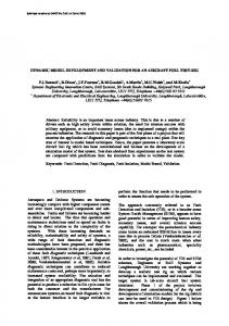
Principal Component Analysis (PCA) for predictor selection would be considered an example of a filter method. In White et al. (2013; p. 11), we described the approach of Li et al. (2008), who used PCA as a method to identify the most relevant predictors for the ABA. PCA is a modelindependent method to reduce feature space and can be easily applied to a set of ALS metrics with the first three Principal Components (PC) typically accounting for the majority of the variance in an ALS point cloud. We provide a sample PCA in Figure 7 for a coastal forest area in British Columbia, Canada. In this case, almost 85% of the variance in the ALS data can be explained by the first three PCs, with the highest component loadings for median height (PC1), coefficient of variation in height (PC2), and canopy cover (% of all returns above mean height; PC3).

40 30 coefficient of variation

20 10

% of all returns above mean height

0 0

5

10

15 Component

20

25

30

Figure 7. Principal components (PC) computed from a set of 30 ALS metrics in a coastal forest of British Columbia, Canada. The majority of the variance within the data can be assigned to a relatively small number of PCs: in this example, the first 3 PCs account for approximately 85% of the total variance in the ALS data. The variables with the highest loadings on each of the first 3 PCs are median height (PC1), coefficient of variation of height (PC2), and canopy cover (% of all returns above mean height; PC3).


23

Lorey’s mean height

Basal area

Gross volume

P90ALS

RumpleALS

P90ALS

HmeanALS

P90ALS

HmeanALS

RumpleALS

HmeanALS

RumpleALS

CoVALS

CoVALS

CoVALS

KurtosisALS

P10ALS

P10ALS

CCmeanALS

SkewnessALS

SkewnessALS P10ALS

HALS

CCmeanALS

10

20

30

KurtosisALS

GALS

SkewnessALS

40

10

20

30

40

KurtosisALS

VALS

CCmeanALS

10

20

30

40

Figure 8. Examples of the variable importance measures derived from random forests (Breiman et al. 2006), and adapted from White et al. (2015b).

In addition to the model-independent approaches for predictor selection such as PCA, some models come with built-in predictor selection possibilities or methods for evaluating predictor importance. For example, the random forests method (See section 3.1; Text Box 1) provides a built-in measure for aiding in predictor selection referred to as variable importance (Breiman 2001). Variable importance is calculated using the mean decrease in accuracy if the values of a given variable are randomly permuted and used as a predictor in the modelling. The greater the decrease in accuracy, the greater the variable importance will be. Figure 8 shows variable importance measures from random forests for predictor variables describing canopy height (e.g. P90ALS), variation in height (e.g. CoVALS), and canopy closure (e.g. CCmeanALS) for estimating Lorey’s mean height, basal area, and gross total volume.

Other studies have selected metrics based on the target information needs and expert judgement (e.g. Asner et al. 2012, Means et al. 2000, Hopkinson and Chasmer 2009). For example, Bouvier et al. (2015) chose only four predictors based on knowledge gained from previous studies concerning the relationship between certain ALS metrics and forest characteristics. The authors selected the mean height of ALS points to describe canopy height, variation in height of ALS points to describe variability of canopy height, proportion of first returns below a specified threshold to describe stand density, and a coefficient of variation of leaf area density from ALS profiles to characterize the vertical structure of a stand.

Table 9. Different resampling approaches for model validation.

24

Method

Description

Data split

Data split partitions the ground plot data into two separate groups: one group is used for training and the other for validation. This method is the most straight-forward, but caution is necessary with regard to the data split. Are the subset samples similar (mean and standard deviation of the forest inventory attribute of interest)? Are rare observations omitted in the training data set? Are there any restrictions one should keep in mind (ground plots in rare forest types, etcetera).

k-fold Cross Validation

This method partitions the ground plot data into k-subsets. Each subset is withheld and the model is trained on the remaining subsets. The withheld subset is used to evaluate model performance. The process is repeated with each subset and the results are summarized in an overall accuracy. k is commonly 3, 5, 7, or 10.

Repeated k-fold Cross Validation

This method repeats the k-fold cross validation a number of times and estimate the overall accuracy as the mean of all repeats.

Leave-one-out cross validation

Leave-one-out is a special case of k-fold Cross Validation. One ground plot is withheld and the model is built using all other ground plots. Repeat for all ground plots.

Bootstrap resampling

In bootstrap resampling, random samples of the available ground plot data are taken with replacement (that is, plots selected for the subset can be selected again in a second or any further selection). In modelling, the bootstrap sample of the same size as the original data set is used for model building, and the remaining plots (that is, those not selected for the current bootstrap; out-of-bag), can be used as independent data to predict on. This sampling—model building—predicting workflow is iterated numerous times (e.g. thousands), and averages of the models’ performances can be used as overall performance.


4.6 How do I evaluate the models I generate? It is critical to evaluate all potential models you generate, as well as their predictions. As noted earlier, regardless of the modelling approach applied, the goal is to develop models that are both biologically plausible and parsimonious using only the most relevant and meaningful predictors for the target attribute(s) of interest. Evaluation of your model also allows you to anticipate how the model is likely to perform when you apply it to new observations (i.e. when you apply the model across your area of interest). In order to quantitatively assess the performance of the established prediction models for forest inventory attributes, a set of performance measures can be computed. These measures describe various aspects of model quality, and caution should be exercised when assessing the accuracy and appropriateness of models based on the results. If you

want to compare the results of your models with reported estimates in other studies, it is essential to carefully read the procedure that was applied and the data included (in the comparative study) when calculating the performance estimates. In general, you can compute performance estimates via different resampling techniques (Table 9) or by using independent validation data (either sampled independently or withheld from use in model development). Since ground plot data are expensive to acquire, it is common to apply resampling methods such as crossvalidation to generate estimates of model performance (Kuhn and Johnson 2013). The statistical software package R (R Core Team 2015) provides a convenient (and no-cost) environment for establishing predictive models for forest inventory attributes. Moreover, you can employ the R package caret (Kuhn 2008) for both model building and evaluation.

Table 10. Summary of common terms used to describe model performance: bias, precision, and accuracy. Term

Definition

Bias

• Bias is defined as “the difference between a population mean of the measurements or test results and an accepted reference or true value” (Bainbridge 1985). • Bias is about the direction of differences between estimates and reference values. Bias results in either an underestimate or an overestimate of the reference value. • A good model should be unbiased, so that an even distribution of underestimates and overestimates leads to an overall bias of zero. • Bias is also termed as “systematic error.” Measurement bias: • Is caused by faulty measuring devices or procedures, and does not decrease with increased sampling effort Sampling bias: • Is the result of unrepresentative sampling of the target population, and does not decrease with increased sampling effort Estimation bias: • Is caused by a biased estimator; average of repeated estimates differs from a true value and decreases with increased sampling effort How is bias measured? • With mean error (ME), also called mean deviation, mean difference, or just “bias”

Precision

• Precision is a measure of the statistical variance of an estimation procedure or, in sampling situations, the spread of the data resulting from the statistical variability present in the sample (Walther and Moore 2005). • Precision is the absence of random error. • A good estimator should be precise so that its estimates show little variation. How is precision measured? • With variance or standard deviation of the estimate

Accuracy

• The overall distance between estimated values and true values. • A good model should be accurate, so that its estimates are as close to the references values as possible. • Accuracy is about the magnitude of the differences between estimates and reference values. How is accuracy measured? • With Mean Square Error (MSE) or Mean Square Deviation (MSD) and Root Mean Square Error (RMSE) • RMSE can be dominated by outliers (i.e. largest differences between estimate and reference value) to avoid this, you can use mean absolute error (MAE) or median of all absolute differences (MAD).


25

In general, there are three terms used to describe model performance: accuracy, precision, and bias. We summarize detailed definitions of these terms and their associated measures in Table 10, and illustrate these concepts in Figure 9.

Regardless of whether you use a parametric or nonparametric method for model development and estimation, the performance measures outlined in Table 11 can be used to evaluate models, and the relative measures can be used to compare model performance between different studies.

Figure 9. An illustration of the concepts of accuracy, precision, and bias.

Table 11. Common measures used to evaluate ABA model performance. Measure

Description

Root Mean Square Error (RMSE)

• An absolute measure of model accuracy • Indicates how close the estimates are to the reference values • Calculated as the square root of the Mean Square Error (MSE) • The mean of the squared differences between estimates and reference values

Relative Root Mean Square Error (RMSE%)

• A relative measure of model accuracy • Scaled by the mean observed value in order to enable comparisons of RMSE between different studies

Mean Error

• An absolute measure of model bias • Calculated as the mean of all differences between estimated and reference values

Relative Mean Error (ME%)

• A relative measure of model bias • Is scaled by the mean observed value in order to enable comparisons of ME between different studies

Equation

ˆ

Note: yi is the observed value and yi is the predicted value for the ien of sample plots; y is the mean value of all observations.

26


5. Generating wall-to-wall predictions 5.1 How do I apply my area-based models across my area of interest?

5.2 How do I exclude areas where models should not be applied?

The grid cell is the fundamental unit of the ABA. Once models have been built using the co-located ALS data metrics and ground measurements, you will need to apply the models to the area of interest using the wall-to-wall metrics generated from the ALS data (see Section 4.3). Recall that these large-area, wall-to-wall metrics are in raster format with each grid cell value representing the metric value for that unit. Raster formats vary and may depend on the software packages you use. The approach for applying the developed models across the area of interest depends on the model type. You can often apply regression equations within a GIS or image processing software package directly, using the package’s inherent mathematical functionality. If you use a modelling approach that does not result in a readily-applied equation, then another software package may be more suitable for the wall-to-wall prediction. For example, the predict function in R could be used, which can handle most model types and can be easily applied to a set of raster layers representing the model inputs (i.e. the ALS metrics). Another example is the R package yaImpute, which has been widely used to build k-NN models and generate wall-to-wall predictions (Crookston and Finley 2007). Yet another option would be to combine the use of Python, R, and GIS software (e.g. ArcGIS, SAGA) to generate wall-to-wall outputs.

Masking of the area of interest is typically required to exclude areas where the developed ABA models should not be applied (e.g. non-forest areas or areas that were recently disturbed). You can use the wall-to-wall ALS metrics to identify areas that should be masked out (Figure 10). For example, you can combine NODATA areas from individual wall-to-wall metric rasters to generate a master NODATA mask. Metrics that are useful for this include the number of returns above a minimum height threshold (e.g. 2 m), the minimum height value for the grid cell, and the percentage of all returns above a minimum height threshold. In Figure 11 we provide an example of a wall-to-wall map of gross merchantable volume, where the no data mask was used to restrict the application of the ABA model.


27

Figure 10. A compiled NODATA mask used to restrict the application of the generated ABA models. Note that if models are being applied by forest type or species group, then an additional mask would be used to identify stands with the appropriate species groupings.

28


Figure 11. A wall-to-wall map of gross merchantable volume generated using the ABA. The NODATA mask in Figure 10 was used to limit the areas to which the model was applied. Information Report FI-X-018

29

5.3 How do I integrate estimates from the area-based approach into a stand-level forest inventory? To maintain maximum flexibility (and useful information), users are encouraged to retain the original ABA gridbased prediction rasters within their GIS data systems. However, recognizing that in the majority of provincial and territorial jurisdictions in Canada (and elsewhere), forest inventory standards require stand-level estimates, we present options for generalizing these rasters to the stand level. To achieve this, you can use stand boundaries from an existing inventory (for alternatives see Section 5.1) to enable the summary of grid-cell predictions to mean stand-level estimates of attributes of interest (see Table 1). Other descriptive statistics can likewise be generated from the grid cells within a given stand (i.e. minimum, maximum, and standard deviation). Prior to computing these stand level statistics, you can apply a buffer (equal to the width of a single grid cell) on the inside of all stand boundaries in order to diminish the negative influence of boundary grid cells (i.e. grid cells that may represent mixed conditions along stand boundaries) on the estimation of within-stand (polygon) means, variances, and other summary statistics (Figure 12). Grid cells within the buffer zone are excluded from the calculation of stand-level summaries. Note that if stands are small (i.e. < 2 ha), buffering may not be a viable option and in that case the grid cell values could be weighted by the proportion of the grid cell area which falls within the stand boundary and use the calculated weights

to generate the stand-level summaries. It is common practice to use the mean or weighted mean value of each attribute as the stand-level estimate of the inventory variable of interest. In contrast to existing stand-level forest inventories that typically provide only a single estimate for the entire stand, the ABA enables within-stand variability to be characterized. Various approaches have been applied to characterize this variability, with the most common being the standard deviation or variance. You can include all stand-level descriptive statistics as separate fields (columns) in an updated stand-level inventory. We recommend caution with respect to characterizing the stand-level uncertainty of area-based estimates. Although it has become common practice to characterize standlevel uncertainty in estimates such as gross total volume or total aboveground biomass using confidence intervals, this approach can result in a marked underestimation of uncertainty and by association, a distorted assessment of ALS-based model performance in the context of an EFI (Magnussen et al. 2016). Confidence intervals are a population-level estimator, meaning they are appropriate for characterizing uncertainty across an entire forest management area, but not for estimating uncertainty for individual forest stands. Magnussen et al. (2016) propose three alternative estimators that are more appropriate for estimating stand-level uncertainty, and end users are encouraged to consider these alternatives if a realistic characterization of stand-level uncertainty in area-based estimates is required.

Figure 12. Existing forest inventory stand boundaries overlaid on rasters of Lorey’s mean height (A) and gross volume (B). The interior of the polygon (hatched) is identified using a 25 m internal buffer applied to the stand boundary. Only cells found under this mask are used to generate stand-level summaries, such as the mean and standard deviation. Boundary grid cells (i.e. those that are found within 25 m of the stand boundary) are thereby excluded from the calculation of stand-level statistics.

30


6. Additional topics on implementing the area-based approach 6.1 How can I create stand boundaries? For obtaining stand boundaries for use in an EFI, you have three main options. You can: • Obtain new boundaries by segmenting ALS data, • Obtain new boundaries by segmenting aerial imagery, or • Use pre-existing stand boundaries

Forest stand boundaries are often required for forest management and planning of operations. A stand should preferably be homogenous in its content, as defined by species composition, tree size, stem density, canopy closure, and site type (Leckie et al. 2003). You can form stands using either operational or biological criteria. Biological stands tend to be smaller and more detailed than stands defined according to operational forest management criteria. The main disadvantage of delineating stand boundaries is the labour-intensive work required to continually update the stands following management activities, and the amount of subjective judgment and manual work required to create stand delineations (Wulder et al. 2008, Hou et al. 2013). Traditionally, stand boundaries have been produced using either visual interpretation or automatic segmentation of aerial imagery (Leckie et al. 2003). You may prefer automated stand delineation using segmentation due to its objectivity. Segmentation algorithms define homogenous regions based on specific properties associated with the remotely sensed data being used, along with criteria for delineated units (e.g. minimum size; Wulder et al. 2008). Different software solutions are available for executing segmentation tasks based on image information (e.g. eCognition, ENVI, ArboLiDAR, MVTec Halcon, Orfeo ToolBox in QGIS, EBImage package in R). Some knowledge and expertise is often required in order to achieve meaningful results from these segmentation algorithms and the software can be expensive. Typically, data used for segmenting forest stands are either very high spatial resolution optical imagery (both air- and spaceborne) or ALS data (Wulder et al. 2008, Koch et al. 2009) In automatic stand delineation, you can often infer variation in tree species or forest type using the spectral information from airborne or satellite imagery; however, imagery lacks information on stand height and density, which are also important criteria for stand delineation. Alternatively, ALS data can capture variation in stand height and density, but lacks tree species and composition information. Therefore, the combination of spectral information from optical data and structural attributes from ALS often produces the most useful stand boundaries for forestry applications

(Diedershagen et al. 2004, Hou et al. 2013). Vastaranta et al. (2014) used the 85th height percentile of the ALS return heights and vegetation density for segmentation. Hou et al. (2013) used attributes predicted with the ABA (volume, basal area) to delineate stands after wall-to-wall estimates were made.

6.2 How can I generate species-specific information? ALS data provide detailed information about forest height and density; however, accurate identification of individual species has not yet been resolved in an operational context. Research into the use of multispectral ALS data (that is, ALS data collected in multiple wavelengths) for individual tree detection and tree species classification is emerging and appears promising (Yu et al. 2017), but questions exist concerning the performance of multispectral ALS data in environments with greater species complexity. Other questions such as the transferability of the species models and the use of this information in the ABA context remain the subject of ongoing research and operational testing (Vauhkonen et al. 2014). The combination of ALS and optical data for obtaining species-specific estimates for forest inventory attributes has been proposed, although care must be taken to ensure that both data sets are acquired approximately at the same time (Packalén and Maltamo 2006, 2007). You can use optical imagery for pre-stratification, prior to the collection of field data, to ensure that the field measurements include all species. Alternatively, you can extract features from the imagery that can be included in the area-based modelling along with ALS metrics. As described above, you may also use available information about tree species or species groups from previous inventories for stratification. The choice of modelling approach for the ABA can also determine how species information is used. For example, parametric regression typically requires individual models (i.e. predictor selection and regression coefficients) for each forest inventory attribute and for each tree species or species group (See Section 2.3). Therefore, and as noted earlier, we recommend pre-stratification of the forest area of interest in order to ensure that each forest type has sufficient ground plots to support the development of predictive models. Næsset (2004b) used aerial imagery for delineating stands and identifying stands dominated by either Scots pine or Norway spruce. Chen et al. (2012) utilized vegetation type maps based on visual interpretation of aerial photographs in biomass estimation. However,


31

using image classification methods for identifying species or species groups (e.g. visual interpretation, supervised or unsupervised classification methods) requires careful consideration, as the use of erroneous species or species groups for stratification can increase the uncertainty of the ABA estimates. As we indicated in Section 4.5, testing for multicollinearity of predictors is a best practice, regardless of the modelling approach selected. When estimating species-specific forest inventory attributes with the ABA, you must test for multicollinearity for each species or species group. With non-parametric approaches, spectral features extracted from aerial imagery that aid in distinguishing tree species can be used directly in the ABA with ALS metrics. In random forests, you could also use species information as categorical variables directly. Depending on the complexity of the tree species assemblages, the number of predictors required for modelling can vary. For example, Packalén and Maltamo (2007) extracted spectral and textural features from aerial imagery, which were included in a nonparametric approach (k-Most-Similar Neighbour or k-MSN) to estimate species-specific forest inventory attributes. In the case of Packalén and Maltamo (2007) predictor selection was not optimized based on identification power, however, correlation between features and proportion of basal area of a species or species group could be used when selecting predictors. When applying non-parametric k-NN approaches, nearest neighbours are sought based on the proximity in relation to the selected predictors. As long as you include variation in species distribution in the ground plot measurements used for model development, non-parametric approaches can produce species-specific forest inventory attributes at the same time for the entire inventory area (Maltamo and Packalén 2015). Depending on information needs associated with species, it is useful to consider estimating the main or dominant tree species along with other forest inventory attributes (Hudak et al. 2008). This requires less information about species distribution and may be obtained more reliably from aerial or high spatial resolution satellite imagery, regardless of the interpretation method used. Tompalski et al. (2014) found that errors in height measurement have more impact on the calculation of individual tree volumes than errors in species, when using species-specific allometric equations. Hence, it is important for end users to recall their need for species information (i.e. are individual tree species or detailed species composition required, or is knowledge of dominant species and/or broader species groups sufficient?), and to allocate their efforts accordingly.

32

To summarize, you will be more successful in determining tree species in forest environments with fewer species or strong physiographic controls on species occurrence, while forest environments with more complex mixtures of tree species will likely remain challenging, even with the advent of multi-spectral ALS systems. By its very nature, the cell size used in the ABA implies a mixture of species (except in pure stands) and for optical data, this is confounded by a mixing of sunlit and shaded crowns as well as canopy gaps within the same ABA grid cell. Thus, if species composition is an inventory requirement and the number of species is large, identification of individual trees and subsequent modelling of tree species is likely required (which could then be summarized at the ABA grid cell level). However, in other environments with more limited species variation, the ABA approach that incorporates species information, as is currently applied in Finland, for example, may suffice.

6.3 How can I derive stem diameter distributions? Most of the ALS research in forest inventory has focused on the estimation of mean characteristics, such as plot or stand mean height or gross total volume. However, from the perspective of both forest value assessment and operative timber harvesting, the prediction of a speciesspecific assortment of stem diameters is by far the most essential issue. For example, you cannot accurately determine the economic value of a forest stand based on total gross volume only. Instead, information on tree species and the stem size distribution is also required to reliably determine the distribution of the total gross volume in various assortments (Holopainen et al. 2010). The timber assortment information can be calculated from speciesspecific DBH distributions. In forest inventory, you obtain attributes such as species-specific stem density, basal area, Lorey’s mean height, and gross total volume. Subsequently, stand-level information is commonly converted into treelevel information through size distribution modelling, which means selecting the appropriate distribution function and the distribution modelling approach (Cao 2004, Siipilehto 2011). Various distributions (e.g. beta, Weibull, and Johnson’s SB) have been applied for estimating speciesspecific size distributions (Päivinen 1980; Kilkki et al. 1989; Maltamo et al. 1995; Siipilehto 1999). Diameter distributions are presented as either unweighted with respect to tree frequency (i.e. DBH-frequency distribution) or weighted with respect to tree basal area (i.e. basal area-DBH distribution) (Gove and Patil 1998). However, weighting will influence the shape of the distribution (Gove and Patil 1998; Siipilehto 1999). Parameters of the size distribution either can be predicted or recovered (Siipilehto and Mehätalo 2013).


Although ALS does not measure diameter directly, the robust statistical relationship between certain ALS metrics and characteristics of stem diameter distributions, allow the latter to be modelled effectively using ALS data (Maltamo and Gobakken 2014). There are many alternative approaches for obtaining diameter distribution using the ABA. When parameters of the distribution function are determined (either predicted or recovered), forest inventory attributes obtained from the ABA are used as model inputs. With a large number of accurately measured plots, you can also build prediction models for diameter distribution parameters using ALS metrics as predictors instead of forest inventory attributes (Gobakken and Næsset 2004). It should be noted that in most of the forest planning systems, stem distribution modelling occurs at the stand level. In the ABA, this requires that the distribution is predicted or recovered after grid-level ABA predictions are aggregated. However, it has been shown that if diameter distributions are predicted for each grid cell, stand-level timber recovery estimates are improved (Siipilehto et al. 2016). You can also predict stem diameter distributions nonparametrically using tree measurements from ground plot data. Field-measured trees can be seen as an empirical stem distribution and with k-NN estimation; it is possible to impute field measured empirical distributions for each grid cell (Maltamo et al. 2009). With this approach, Packalén and Maltamo (2008) outperformed the Weibull-function parameter prediction method. However, imputation of the empirical stem distribution easily adds to the amount of the data to be saved for each prediction cell, and care must be taken to ensure that the modelling data are sufficiently comprehensive. Research into stem size distributions continues to evolve. Magnussen and Renaud (2016) demonstrated how a relative frequency distribution of canopy heights derived from ALS data can be used to improve the estimation of stem size distributions. Using multi-dimensional scaling, the authors present a scalable approach—meaning the approach enables generation of both stand- and stratum-level stem size distributions.

6.4 How can I make use of the intra-stand variation provided by the area-based approach? The ABA provides estimates of forest inventory attributes for each grid cell. As we noted in Section 5.3, these gridcell estimates can be aggregated in some way to generate an estimate for the forest stand. However, for some forestry applications, it is worthwhile to take advantage of the grid cell-level information rather than using aggregated stand attributes. In general, EFI raster layers of forest inventory attributes describe variation in forest structure with far more detail than stand-level information. If some preexisting stand boundaries are used, raster layers reveal within-stand variation. On the other hand, these raster layers can minimize intra-stand variation if you use them to derive stand boundaries using automated segmentation approaches (e.g. Hou et al. 2013), as described in Section 6.1. Automatic segmentation may allow dynamic stand boundaries to be defined “on the fly” for specific forest operations. For example, forest stands that have similar stand characteristics in basal area, site quality, and growth may all reach maturity for harvest at similar times, thereby allowing for similar management prescriptions. You can use raster layers derived from the ABA to create dynamic stand harvest boundaries. In this case, stand boundaries are determined by the probability that the grid cell is sufficiently mature for harvest, with probabilities estimated from a model that incorporates information from a series of ABA rasters. You can also utilize ABA raster layers of forest inventory attributes to provide a more detailed estimation of forest structure, such as in the characterization of stem diameter distributions (See 5.4).


33

7. Resources Online tutorials:

Software:

The Remote Sensing Applications Centre of the US Forest Service has generated many online ALS-related tutorials. These tutorials cover a range of topics, including an introduction to modelling with R.

Packages in R useful for manipulating ALS data and for spatial operations:

• https://www.fs.fed.us/eng/rsac/lidar_training/

The rapidlasso website (LAStools) provides many online tutorials and videos. • https://rapidlasso.com/category/tutorials/

Documents: The best practices guide referred to herein (White et al., 2013), is available for download in both English and French language versions from the Canadian Forest Service bookstore: • https://cfs.nrcan.gc.ca/publications?id=34887 • https://cfs.nrcan.gc.ca/publications?id=35375

• lidR: R package for airborne LiDAR data manipulation

and visualisation for forestry application (https://github. com/Jean-Romain/lidR, https://CRAN.R-project.org/ package=lidR) • sp: Classes and Methods for Spatial Data

(https://CRAN.R-project.org/package=sp) • sf: Simple features for R (https://CRAN.R-project.org/

package=sf); Package for handling all kinds of spatial vector data in R • raster: Geographic Data Analysis and Modelling

(https://CRAN.R-project.org/package=raster); Useful package for all raster operations in R Packages in R that are useful for statistical modelling and the ABA: • randomForest (https://cran.r-project.org/web/packages/

randomForest/randomForest.pdf) • yaimpute (https://cran.r-project.org/web/packages/

yaImpute/yaImpute.pdf) • caret (https://cran.r-project.org/web/packages/caret/index.

html)

8. Acknowledgements We thank the Canadian Wood Fibre Centre (CWFC) of the Canadian Forest Service, Natural Resources Canada for funding support that facilitated the preparation of this best practices guide. Our gratitude also extends to the many staff of the CWFC and its partners who have contributed to the Enhanced Forest Inventotry project. Mikko Vastaranta and Ninni Saarinen owe their contribution

34

to this project to the Centre of Excellence in Laser Scanning Research (decision number 272195) within the Academy of Finland. We also thank Giona Matasci for his help with the preparation of the detailed figures in the guide. Joan Luther and Chris Bater are thanked for their insightful comments on earlier versions of this document.


9. References Akaike, H. 1973. Information theory and an extension of the maximum likelihood principle. In Second International Symposium on Information Theory, (Academiai Kiado, Budapest, Hungary), pp. 267–281. Asner, G.P., Mascaro, J., Muller-Landau, H.C., Vieilledent, G., Vaudry, R., Rasamoelina, M., Hall, J.S., van Breugel, M. 2012. A universal airborne LiDAR approach for tropical forest carbon mapping. Oecologia, 168(4): 1147–1160. Bainbridge, T. R. 1985. The Committee on Standards: precision and bias. ASTM Standardization News 13: 44–46.

Diedershagen, O., Koch, B., Weinacker, H. 2004. Automatic segmentation and characterisation of forest stand parameters using airborne lidar data, multispectral and fogis data. International Archives of Photogrammetry, Remote Sensing and Spatial Information Sciences, 36: 208–212. Eskelson, B.N.I., Temesgen, H., Lemay, V., Barrett, T.M., Crookston, N.L., Hudak, A.T. 2009. The roles of nearest neighbour methods in imputing missing data in forest inventory and monitoring databases. Scandinavian Journal of Forest Research, 24(3), 235–246.

Bater, C.W., Wulder, M.A., Coops, N.C., Nelson, R.F., Hilker, T., Næsset, E. (2011). Stability of sample-based scanning-LiDARderived vegetation metrics for forest monitoring. Transactions on Geoscience and Remote Sensing 49, 2385–2392.

Frazer, G. W., Magnussen, S., Wulder, M. A., Niemann, K. O. 2011. Simulated impact of sample plot size and co-registration error on the accuracy and uncertainty of LiDAR-derived estimates of forest stand biomass. Remote Sensing of Environment, 115(2): 636–649.

Breidenbach, J., Næsset, E., Lien, V., Gobakken, T., Solberg, S. 2010a. Prediction of species specific forest inventory attributes using a nonparametric semi-individual tree crown approach based on fused airborne laser scanning and multispectral data. Remote Sensing of Environment, 114(4): 911–924.

Franco-Lopez, H., Ek., A.R., Bauer, M.E. 2001. Estimation and mapping of forest stand density, volume, and cover type using the k-nearest neighbours method. Remote Sensing of Environment, 77: 251–274.

Breidenbach, J., Nothdurft, A., Kändler, G. 2010b. Comparison of nearest neighbour approaches for small area estimation of tree species-specific forest inventory attributes in central Europe using airborne laser scanner data. European Journal of Forest Research, 129(5): 833–846. Breiman, L. 2001. Random forests. Machine Learning 45(1): 5–32. Brosofske, K.D., Froese, R.E., Falksowski, M.J., Banskota, A. 2014. A review of methods for mapping and prediction of inventory attributes for operational forest management. Forest Science, 60(2): 733–756. Bouvier, M., Durrieu, S., Fournier, R. A., Renaud, J.-P. 2015. Generalizing predictive models of forest inventory attributes using an area-based approach with airborne LiDAR data. Remote Sensing of Environment, 156: 322–334. Cao, Q.V. 2004. Predicting parameters of a Weibull function for modelling diameter distribution. Forest Science, 50(5): 682–685. Chasmer, L., Hopkinson, C., Treitz, P.. 2006. Examining the influence of changing laser pulse repetition frequencies on conifer forest canopy returns. Photogrammetric Engineering and Remote Sensing 72(12): 1359–1367. Chen, Q., Vaglio Laurin, G., Battles, J.J., Saah, D. 2012. Integration of airborne lidar and vegetation types derived from aerial photography for mapping aboveground live biomass. Remote Sensing of Environment 121: 108-117. Chirici, G., Mura, M., McInerney, D., Py, N., Tomppo, E.O., Waser, L. T., Travaglini, D., McRoberts, R. E. 2016. A meta-analysis and review of the literature on the k-Nearest Neighbours technique for forestry applications that use remotely sensed data. Remote Sensing of Environment, 176: 282–294. Crookston, N.L., Finley, A.O. 2007. yaImpute: An R Package for k-NN Imputation. Journal of Statistical Software, 23(10):1–16. Demaerschalk, J.P., Kozak, A. 1974. Suggestions and criteria for more effective regression sampling. Canadian Journal of Forest Research, 4: 341–348. Deo, R., Froese, R.E., Falkowski, M.J., Hudak, A.T. 2016. Optimizing variable radius plot size and lidar resolution to model standing volume in coniferous forests. Canadian Journal of Remote Sensing, 42: 428–442.

Gobakken, T., Næsset, E. 2004. Estimation of diameter and basal area distributions in coniferous forest by means of airborne laser scanner data. Scandinavian Journal of Forest Research, 19(6): 529–542. Gobakken, T., Næsset, E. 2008. Assessing effects of laser point density, ground sampling intensity, and field sample plot size on biophysical stand properties derived from airborne laser scanner data. Canadian Journal of Forest Research, 38: 1095–1109. Gobakken, T., Næsset, E. 2009. Assessing effects of positioning errors and sample plot size on biophysical stand properties derived from airborne laser scanner data. Canadian Journal of Forest Research, 39: 1036–1052. Gobakken, T., Korhonen, L., Næsset, E. 2013. Laser-assisted selection of field plots for an area-based forest inventory. Silva Fennica, 47(5): 1–20. Goodwin, N.R., Coops, N.C., Culvenor, D.S. 2006. Assessment of forest structure with airborne LiDAR and the effects of platform altitude, Remote Sensing of Environment, 103: 140–152. Gove, J.H., Patil, G.P. 1998. Modelling the basal area-size distribution of forest stands: a compatible approach. Forest Science, 44: 285–297 Grafström, A., Ringvall, A.H., 2013. Improving forest field inventories by using remote sensing in novel sampling designs. Canadian Journal of Forest Research, 43: 1015-1022. Gregoire, T. G., Næsset, E., McRoberts, R. E., Ståhl, G., Andersen, H.-E., Gobakken, T., Ene, L., Nelson, R. 2016. Statistical rigor in LiDAR-assisted estimation of aboveground forest biomass. Remote Sensing of Environment, 173: 98–108. Hawbaker, T., Keuler, N., Lesak, A., Gobakken, T., Contrucci, K., Radeloff, V. 2009. Improved estimates of forest vegetation structure and biomass with a LiDAR-optimized sampling design, Journal of Geophysical Research, 114(4): 1–11. Heurich, M., Thoma, F. 2008. Estimation of forestry stand parameters using laser scanning data in temperate, structurally rich natural European beech (Fagus sylvatica) and Norway spruce (Picea abies) forests. Forestry, 81(5), 645–661. Holopainen, M., Vastaranta, M., Rasinmäki, J., Kalliovirta, J., Mäkinen, A., Haapanen, R., Melkas, T., Yu, X. and Hyyppä, J., 2010. Uncertainty in timber assortment estimates predicted from forest inventory data. European journal of forest research, 129(6): 1131–1142.


35

Hopkinson, C. 2007. The influence of flying altitude, beam divergence, and pulse repetition frequency on laser pulse return intensity and canopy frequency distribution. Canadian Journal of Remote Sensing, 33(4): 312–324.

Leckie, D., Gougeon, F., Walsworth, N., Paradine, D. 2003. Stand delineation and composition estimation using semiautomated indiviual tree crown analysis. Remote Sensing of Environment, 85: 355–369.

Hopkinson, C., Chasmer, L. 2009. Testing LiDAR models of fractional cover across multiple forest ecozones. Remote Sensing of Environment 113(1): 275-288.

Lefsky, M.A., Hudak, A.T., Cohen, W.B., Acker, S.A. 2005. Patterns of covariance between forest stand and canopy structure in the Pacific Northwest. Remote Sensing of Environment, 95(4): 517- 531.

Hou Z., Xu Q., Nuutinen T., Tokola T. 2013. Extraction of remote sensing based forest management units in tropical forest. Remote Sensing of Environment, 130: 1-10. Hudak, A. T., Crookston, N. L., Evans, J. S., Falkowski, M. J., Smith, A. M., Gessler, P. E., Morgan, P. 2006. Regression modelling and mapping of coniferous forest basal area and tree density from discrete-return lidar and multispectral satellite data. Canadian Journal of Remote Sensing, 32(2): 126–138. Hudak, A.T., Crookston, N.L., Evans, J.S., Hall, D.E., Falkowski, M.J. 2008. Nearest neighbour imputation of species-level, plot-scale forest structure attributes from LiDAR data. Remote Sensing of Environment, 112(5), 2232–2245. Hudak, A.T., Haren, A.T., Crookston, N.L., Liebermann, R.J., Ohmann, J.L. 2014. Imputing Forest Structure Attributes from Stand Inventory and Remotely Sensed Data in Western Oregon, USA. Forest Science, 60: 253–269. Immitzer, M., Stepper, C., Böck, S., Straub, C., Atzberger. C. 2016. Use of WorldView-2 stereo imagery and National Forest Inventory data for wall-to-wall mapping of growing stock. Forest Ecology and Management, 359:232–246. Jakubowski, M.K., Guo, Q., Kelly, M. 2013. Tradeoffs between LiDAR pulse density and forest measurement accuracy. Remote Sensing of Environment, 103: 245–253. Junttila, V., Finley, A.O., Bradford, J.B., Kauranne, T. 2013. Strategies for minimizing sample size for use in airborne LiDARbased forest inventory. Forest Ecology and Management, 292(5): 75–85. Kaartinen, H., Hyyppä, J., Yu, X., Vastaranta, M., Hyyppä, H., Kukko, A., Holopainen, M. et al. 2012. An International Comparison of Individual Tree Detection and Extraction Using Airborne Laser Scanning. Remote Sensing 2012, 4, 950–974. Keränen, J., Maltamo, M., Packalén, P. 2016. Effect of flying altitude, scanning angle and scanning mode on the accuracy of the ALS based forest inventory. International Journal of Applied Earth Observation and Geoinformation, 52: 349–360. Koch, B., Straub, C., Dees, M., Wang, Y., Weinacker, H. 2009. Airborne laser data for stand delineation and information extraction. International Journal of Remote Sensing, 30(4): 935–963. Kuhn, M. 2008. Building predictive models in R using the caret package. Journal of Statistical Software 28(5): 1–26.

36

Lemay, V. M., Temesgen, H. (2005). Comparison of Nearest Neighbour Methods for Estimating Basal Area and Stems per Hectare Using Aerial Auxiliary Variables. Forest Science, 51(2), 109–119. Liaw, A., Wiener, M. 2002. Classification and regression by randomForest. R News, 2/3: 18–22. Li, Y. Andersen, H.-E., McGaughey, R. 2008. A Comparison of statistical methods for estimating forest biomass from light detection and ranging. Western Journal of Applied Forestry, 23(4): 223–231. Lim, K., Hopkinson, C., Treitz, P. 2008. Examining the effects of sampling point densities on laser canopy height and density metrics. The Forestry Chronicle, 84(6): 876–885. Luther, J.E., Skinner, R., Fournier, R.A., van Lier, O.R., Bowers, W.W., Côté, J.-F., Hopkinson, C., and Moulton, T. 2014. Predicting wood quantity and quality attributes of balsam fir and black spruce using airborne laser scanner data, Forestry, 87: 313-326. Magnussen, S., Boudewyn, P. 1998. Derivations of stand heights from airborne laser scanner data with canopy-based quantile estimators. Canadian Journal of Forest Research, 28: pp. 1016–1031. Magnussen, S., Næsset, E., Gobakken, T. 2013. Prediction of treesize distributions and inventory variables from cumulants of canopy height distributions. Forestry, 86(5): 583-595. Magnussen, S., Frazer, G., Penner, M. 2016. Alternative meansquared error estimators for synthetic estimators of domain means. Journal of Applied Statistics, 43: 2550–2573. Magnussen, S., Renaud, J.-P. 2016. Multidimensional scaling of first-return airborne laser echoes for prediction and modelassisted estimation of a distribution of tree stem diameters. Annals of Forest Science, 73: 1089–1098. Maltamo, M., Eerikäinen, K. 2001. The Most Similar Neighbour Reference in the Yield Prediction of Pinus kesia Stand in Zambia. Silva Fennica, 35(4): 437–451. Maltamo, M, Puumalainen, J., Päivinen, R. 1995. Comparison of Beta and Weibull functions for modelling basal area diameter distribution in stands of Pinus sylvestris and Picea abies. Scandinavian Journal of Forest Research,10: 284-295.

Kuhn, M., Johnson, K. 2013. Applied Predictive Modelling. New York, NY: Springer.

Maltamo, M., Malinen, J., Kangas, A., Härkönen, S., Pasanen, A. M. 2003. Most similar neighbour-based stand variable estimation for use in inventory by compartments in Finland. Forestry, 76(4), 449–463.

Latifi, H., Nothdurft, A., Koch, B. 2010. Non-parametric prediction and mapping of standing timber volume and biomass in a temperate forest: application of multiple optical/LiDAR-derived predictors. Forestry, 83(4), 395–407.

Maltamo, M., Eerikainen, K., Pitkanen, J., Hyyppa, J., Vehmas, M. 2004. Estimation of timber volume and stem density based on scanning laser altimetry and expected tree size distribution functions. Remote Sensing of Environment, 90(3), 319–330.

Latifi, H., Fassnacht, F. E., Hartig, F., Berger, C., Hernández, J., Corvalán, P., Koch, B. 2015. Stratified aboveground forest biomass estimation by remote sensing data. International Journal of Applied Earth Observations and Geoinformation, 38, 229–241.

Maltamo, M., Næsset, E., Bollandsås, O. M., Gobakken, T., Packalén, P. 2009. Non-parametric prediction of diameter distributions using airborne laser scanner data. Scandinavian Journal of Forest Research, 24(6): 541–553.


Maltamo, M., Bollandsås, O. M., Næsset, E., Gobakken, T., Packalén, P. 2011. Different plot selection strategies for field training data in ALS-assisted forest inventory. Forestry, 84(1): 23-31. Maltamo, M., Gobakken, T. 2014. Predicting tree diameter distributions. Chapter 9 in M. Maltamo, E. Næsset, J. Vauhkonen (Eds.), Forestry Applications of Airborne Laser Scanning: Concepts and Case Studies, Dordrecht: Springer. 464 p. Maltamo, M., Packalén, P. 2015. Species-specific management inventory in Finland. Chapter 12 In Maltamo, M., Næsset, E.,Vauhkonen, J. Forestry Applications of Airborne Laser Scanning, Concepts and Case Studies, New York, NY: Springer. McGaughey, R.J. 2016. FUSION/LDV: Software for LIDAR data analysis and visualization (October 2016 FUSION Version 3.60+. United States Department of Agriculture, Forest Service, Pacific Northwest Research Station. Available online: http://forsys.cfr. washington.edu/fusion/FUSION_manual.pdf (Accessed February 27, 2017). McRoberts, R.E., Domke, G.M., Chen, Q., Næsset, E., Gobakken, T. 2016. Using genetic algorithms to optimize k-Nearest Neighbours configurations for use with airborne laser scanning data. Remote Sensing of Environment, 184: 387–395. Means, J.E., Acker, S.A., Fitt, B.J., Renslow, M., Emerson, L., Hendrix, C.J. 2000. Predicting Forest Stand characteristics with Airborne Scanning Lidar. Photogrammetric Engineering & Remote Sensing 66(11): 1367–1371.

Næsset, E. 2011. Estimating above-ground biomass in young forests with airborne laser scanning. – International Journal of Remote Sensing, 32: 473–501. Næsset, E. 2015. Area-based inventory in Norway – from innovations to operational reality. Chapter 11 in Maltamo, M., Næsset, E.,Vauhkonen, J. Forestry Applications of Airborne Laser Scanning, Concepts and Case Studies, New York, NY: Springer. Næsset, E., Bjerknes, K.-O. 2001. Estimating tree heights and number of stems in young forest stands using airborne laser scanner data. Remote Sensing of Environment, 78: 328–340. Næsset, E., Bollandsas, O. M., Gobakken, T., Bollandsås, O. M. 2005. Comparing regression methods in estimation of biophysical properties of forest stands from two different inventories using laser scanner data. Remote Sensing of Environment, 94(4): 541–553. Nelson, R. 2013. How did we get here? An early history of forestry LiDAR. Canadian Journal of Remote Sensing, 39: S1–S12. Nurminen, K., Karjalainen, M., Yu, X., Hyyppä, J., Honkavaara, E. 2013. Performance of dense digital surface models based on image matching in the estimation of plot-level forest variables. ISPRS Journal of Photogrammetry and Remote Sensing, 83: 104–115. Ohmann, J.L., Gregory, M.J. 2002. Predictive mapping of forest composition and structure with direct gradient analysis and nearest-neighbour imputation in coastal Oregon, USA. Canadian Journal of Forest Research, 32:725–741.

Melville, G., Stone, C. 2016. Optimising nearest neighbour information–a simple, efficient sampling strategy for forestry plot imputation using remotely sensed data. Australian Forestry, 79(3): 217–228.

Packalén, P., Maltamo, M. 2006. Predicting the Plot Volume by Tree Species Using Airborne Laser Scanning and Aerial Photographs. Forest Science, 52(6): 611–622.

Montaghi, A. 2013. Effect of scanning angle on vegetation metrics derived from a nationwide airborne laser scanning acquisition. Canadian Journal of Remote Sensing, 39:S152–S173.

Packalén, P., Maltamo, M. 2007. The k-MSN method for the prediction of species-specific stand attributes using airborne laser scanning and aerial photographs. Remote Sensing of Environment, 109(3): 328-341.

Montgomery, D.C., Peck, E.A., Vining, G.G. 2006. Introduction to linear regression analysis. John Wiley & Sons, Inc.

Packalén, P. and Maltamo, M. 2008. Estimation of species-specific diameter distributions using airborne laser scanning and aerial photographs. Canadian Journal of Forest Research, 38: 1750–1760.

Morsdorf, F., Frey, O., Meier, E., Itten, K.I., Allgöwer. 2008. Assessment of the influence of flying altitude and scan angle on biophysical vegetation products dervied from airborne laser scanning. International Journal of Remote Sensing, 29: 1387–1406.

Packalén, P., Suvanto, A., Maltamo, M. 2009. A two-stage method to estimate species-specific growing stock. Photogrammetric Engineering & Remote Sensing, 75(12): 1451–1460.

Muinonen, E., Maltami, M. Hyppänen, H., Vainikainen, V. 2001. Forest Stand Characteristics Estimation Using a Most Similar Neighbour Approach and Image Spatial Structure Information. Remote Sensing of Environment 78: 223–228.

Packalén, P., Temesgne, H., Maltamo, M. 2012. Variable selection strategies for nearest neighbor imputation methods used in remote sensing based forest inventory. Canadian Journal of Remote Sensing, 38(5): 1–13.

Næsset, E. 1997. Estimating timber volume of forest stands using airborne laser scanner data. Remote Sensing of Environment, 61(2): 246–253.

Penner, M., Pitt, D.G., Woods, M.E. 2013. Parametric versus nonparametric LiDAR models for operational forest inventory in boreal Ontario. Canadian Journal of Remote Sensing, 39(5): 426–443.

Næsset, E. 2002. Predicting forest stand characteristics with airborne scanning laser using a practical two-stage procedure and field data. Remote Sensing of Environment, 80(1): 88–99. Næsset, E. 2004a. Practical large-scale forest stand inventory using a small-footprint airborne scanning laser. Scandinavian Journal of Forest Research, 19:164–179. Næsset, E. 2004b. Accuracy of forest inventory using airborne laser scanning: evaluating the first nordic full-scale operational project. Scandinavian Journal of Forest Research, 19:554–557. Næsset, E. 2009. Influence of terrain model smoothing and flight and sensor configurations on detection of small pioneer trees in the boreal-alpine transition zone utilizing height metrics derived from airborne scanning lasers. Remote Sensing of Environment, 113: 2210–2223.

Penner, M., Woods, M., Pitt, D. 2015. A comparison of airborne laser scanning and image point cloud derived tree size class distribution models in boreal Ontario. Forests, 6(11): 4034–4054. Ruiz, L.A., Hermosilla, T., Mauro, F., Godino, M. 2014. Analysis of the influence of plot size and LiDAR density on forest structure attribute estimates. Forests, 5: 936–951. Shin, J., Temesgen, H., Strunk, J.L., Hilker, T. 2016. Comparing modelling methods for predicting forest attributes using LiDAR metrics and ground measurements. Canadian Journal of Remote Sensing, 42(6): 739–765.


37

Siipilehto, J. 1999. Improving the accuracy of predicted basal-area diameter distribution in advanced stands by determining stem number. Silva Fennica, 33(4): 281-301. Siipilehto, J. 2011. Local prediction of stand structure using linear prediction theory in Scots pine-dominated stands in Finland. Silva Fennica, 45(4): 669–692. Siipilehto, J., Mehtätalo, L. 2013. Parameter recovery vs. parameter prediction for the Weibull distribution validated for Scots pine stands in Finland. Silva Fennica, 47(4): 1–22. Siipilehto, J., Lindeman, H., Vastaranta, M., Yu, X.,Uusitalo, J. 2016. Reliability of the predicted stand structure for clear-cut stands using optional methods: airborne laser scanning-based methods, smartphone-based forest inventory application Trestima and preharvest measurement tool EMO. Silva Fennica, 50(3): 1–24. Sprugel, D.G. 1983. Correcting for bias in log-transformed allometric equations. Ecology 64, 209–210. Stage, A. R. & Crookston, N. L. (2007). Partitioning error components for accuracy-assessment of near-neighbor methods of imputation. Forest Science, 53, 62–72. Strunk, J., Temesgen, H., Andersen, H.-E., Flewelling, J.P., Madsen, L. 2012. Effects of lidar pulse density and sample size on a model-assisted approach to estimate forest inventory variables. Canadian Journal of Remote Sensing, 38: 644-654. Tompalski, P., Coops, N.C., White, J.C., Wulder, M.A. 2014. Simulating the impacts of error in species and height upon tree volume derived from airborne laser scanning data. Forest Ecology and Management, 327:167–177. Tompalski, P., Coops, N.C., White, J.C., Wulder, M.A. 2015. Enriching ALS-derived area-based estimates of volume through tree-level downscaling. Forests, 6(8), 2608–2630. Tomppo, E., Kuusinen, N., Makisara, K., Katila, M., McRoberts, R.E. 2016. Effects of field plot configurations on the uncertainties of ALS-assisted forest resource estimates. Scandinavian Journal of Forest Research. Treitz, P., Lim, K., Woods, M., Pitt, D., Nesbitt, D., Etheridge, D. 2012. LiDAR sampling density for forest resource inventories in Ontario, Canada. Remote Sensing, 4: 830–848. Vauhkonen, J., Ene, L., Gupta, S., Heinzel, J., Holmgren J., Pitkänen, J., Solberg, S., Wang, Y., Weinacker, H., Hauglin, K.M., Lien V., Packalén, P., Gobakken, T., Koch, B., Næsset, E., Tokola, T., Maltamo, M. (2012). Comparative testing of single-tree detection algorithms under different types of forest. Forestry 85(1):27-40. Vastaranta, M., Wulder, M.A., White, J.C., Pekkarinen, A., Tuominen, S., Ginzler, C., Kankare, V., Holopainen, M., Hyyppä, J. Hyyppä, H. 2013. Airborne laser scanning and digital stereo imagery measures of forest structure: comparative results and implications to forest mapping and inventory update. Canadian Journal of Remote Sensing, 39:382–395 Vastaranta, M., Saarinen, N., Kankare, V., Holopainen, M., Kaartinen, H., Hyyppa, J., and Hyyppä, H. 2014. Multisource single-tree ¨ inventory in the prediction of tree quality variables and logging recoveries. Remote Sensing, 6: 3475–3491. Véga, C., Renaud, J.-P., Durrieu, S., Bouvier, M. 2016. On the interest of penetration depth, canopy area, and volume metrics to improve lidar-based models of forest parameters. Remote Sensing of Environment, 175: 32–42. van Ewijk, K.Y., Treitz, P.M., Scott, N.A. 2011. Characterizing forest succession in Central Ontario using LiDAR-derived indices. Photogrammetric Engineering and Remote Sensing, 77(3), 261–269.

38

Vauhkonen, J., Ørka, H. O., Holmgren, J., Dalponte, M., Heinzel, J., Koch, B. 2014. Tree species recognition based on airborne laser scanning and complementary data sources. Chapter 7 in M. Maltamo, E. Næsset, J. Vauhkonen (Eds.), Forestry Applications of Airborne Laser Scanning: Concepts and Case Studies, Dordrecht: Springer. 464 p. Villikka, M., Packalén, P., Maltamo, M. 2012. The suitability of leafoff airborne laser scanning data in an area-based forest inventory of coniferous and deciduous trees. Silva Fennica, 46(1): 99-110 Walther, B.A., Moore, J.L. 2005. The concepts of bias, precision and accuracy, and their use in testing the performance of species richness estimators, with a literature review of estimator performance. Ecography, 28 (6):815–829. White, J.C., Wulder, M.A., Varhola, A., Vastaranta, M., Coops, N.C., Cook, B.D., Pitt, D, Woods, M. 2013. A best practices guide for generating forest inventory attributes from airborne laser scanning data using the area-based approach. Information Report FI-X-10. Canadian Forest Service, Canadian Wood Fibre Centre, Pacific Forestry Centre, Victoria, B.C. 50 p. Available online: http://www.cfs.nrcan.gc.ca/pubwarehouse/pdfs/34887. pdf [Accessed February 13, 2017]. White, J.C., Arnett, J.T.T.R., Wulder, M.A., Tompalski, P., Coops, N.C. 2015a. Evaluating the impact of leaf-on and leaf-off airborne laser scanning data on the estimation of forest inventory attributes with the area-based approach. Canadian Journal of Forest Research, 45: 1498–1513. White, J.C., Stepper, C., Tompalski, P., Coops, N.C., Wulder, M.A. 2015b. Comparing ALS and image-based point cloud metrics and modelled forest inventory attributes in a complex coastal forest environment. Forests, 6(10): 3704-3732. White, J.C., Coops, N.C., Wulder, M.A., Vastaranta, M., Hilker, T., Tompalski, P. 2016. Remote sensing for enhancing forest inventories: A review. Canadian Journal of Remote Sensing, 42(5): 619–641. Woods, M., Pitt, D., Penner, M., Lim, K., Nesbitt, D., Etheridge, D., Treitz, P. 2011. Operational implementation of a LiDAR inventory in Boreal Ontario. The Forestry Chronicle, 87(4): 512–528. Wulder, M. A., White, J. C., Hay, G. J., Castilla, G. 2008. Towards Automated Segmentation of Forest Inventory Polygons on High Spatial Resolution Satellite Imagery. The Forestry Chronicle, 84(2):221-230. Yu, X., Hyyppä, J., Vastaranta, M., Holopainen, M., Viitala, R. 2011. Predicting individual tree attributes from airborne laser point clouds based on the random forests technique. ISPRS Journal of Photogrammetry and Remote Sensing, 66(1), 28–37. Yu, X., Hyyppä, J., Karjalainen, M., Nurminen, K., Karila, K., Vastaranta, M., Kankare, V., Kaartinen, H., Holopainen, M., Honkavaara, E., Kukko, A., Jaakkola, A., Liang, X., Wang, Y., Hyyppä, H., Katoh, 2015. M. Comparison of laser and stereo optical, sar and insar point clouds from air- and space-borne sources in the retrieval of forest inventory attributes. Remote Sensing, 7(12), 15933-15954. Yu, X., Hyyppä, J., Litkey, P., Kaartinen, H., Vastaranta, M., Holopainen, M. 2017. Single-sensor solution to tree species classification using multispectral airborne laser scanning. Remote Sensing, 9(2): 108. Zald, H.S.J., Ohmann, J.L. Roberts, H.M., Gregory, M.J., Henderson, E.B., McGaughey, R.J., Braaten, J. 2014. Influence of lidar, Landsat imagery, disturbance history, plot location accuracy, and plot size on accuracy of imputation maps of forest composition and structure. Remote Sensing of Environment, 143: 26–38. Zellner, A. 1962. An Efficient Method for Estimating Seemingly Unrelated Regressions and Tests for Aggregation Bias. Journal of the American Statistical Association, 57(298), 348–368.


For more information about the Canadian Forest Service, visit our Web site or contact any of the following Canadian Forest Service establishments

cfs.nrcan.gc.ca 4 1 2 5 1 3

6

Canadian Forest Service Contacts 1

Atlantic Forestry Centre P.O. Box 4000 1350 Regent Street South Fredericton, NB E3B 5P7 Tel.: 506-452-3500 Fax: 506-452-3525 cfs.nrcan.gc.ca/regions/afc Atlantic Forestry Centre Corner Brook Office P.O. Box 960 26 University Drive Corner Brook, NL A2H 6J3 Tel.: 709-637-4900 Fax: 709-637-4910

2

Laurentian Forestry Centre 1055 du P.E.P.S. P.O. Box 10380 Sainte-Foy Stn. Québec, QC G1V 4C7 Tel.: 418-648-3335 Fax: 418-648-5849 cfs.nrcan.gc.ca/regions/lfc

3

Great Lakes Forestry Centre 1219 Queen St. East Sault Ste. Marie, ON P6A 2E5 Tel.: 705-949-9461 Fax: 705-759-5700 cfs.nrcan.gc.ca/regions/glfc

4

Northern Forestry Centre 5320-122nd Street Edmonton, AB T6H 3S5 Tel.: 403-435-7210 Fax: 403-435-7359 cfs.nrcan.gc.ca/regions/nofc

5

Pacific Forestry Centre 506 West Burnside Road Victoria, BC V8Z 1M5 Tel.: 250-363-0600 Fax: 250-363-0775 cfs.nrcan.gc.ca/regions/pfc

6

Headquarters 580 Booth St., 8th Fl. Ottawa, ON K1A 0E4 contact-contactez.nrcan-rncan.gc.ca cfs.nrcan.gc.ca/regions/nrc Canadian Wood Fibre Centre 580 Booth St., 7th Fl. Ottawa, ON K1A 0E4 cwfc.nrcan.gc.ca

To order publications online, visit the Web site “Canadian Forest Service Publications” at

cfs.nrcan.gc.ca/publications

A model development and application guide for generating an ...

A model development and application guide for generating an ...

Suggest Documents

A Model for Affective Computing Application Development

Development and Application of an Oral Challenge Mouse Model for ...

Development, Evaluation, and Application of an In Silico Model for ...

Development and Application of an Oral Challenge Mouse Model for ...

the development and application of an injury prediction model for ...

An Empirical model for Generating the IV Characteristics for a

DEVELOPMENT AND APPLICATION OF A BIOENERGETICS MODEL ...

AN AUTOMATED MODEL FOR GENERATING A ... - ITC Digital Library

development and application of a physical model for ... - AMS Dottorato

Development and application of a model for robust, cost ... - esanalysis

Development and Application of a Screening Model for Simulating

Development of an Influenza A Master Virus for Generating High

An Efficient Objective Quality Model for Agile Application Development

A Computational Approach for Generating Toulmin Model ...

A New Model for Generating Multimodal Referring

A Computational Approach for Generating Toulmin Model ...

A Model for Teaching Mobile Application Development for ... - FedCSIS

Development and Application of an Experimental Model ... - CiteSeerX

Development and Application of an Energy Model ...

H Model for Handheld Application Development

Modified W Model for Handheld Application Development

DYNAMIC MODEL DEVELOPMENT AND VALIDATION FOR AN ...

Generating and Model Checking a Hierarchy of

an application guide - Porterfield