A Model for Computer Design - IEEE Computer Society

The Lagrange multiplier method unravels the configuration design problem. It guarantees a global solution that optimizes device speeds and main memory size.

A Model for Computer

Configuration

Design

Kishor S. Trivedi Duke University

Robert E. Kinicki Worcester Polytechnic Institute

Computer system performance depends upon interactions among the software components, the hardware components, and the user workload. Understanding the nature of these interdependences requires collecting experimental data and developing a mechanism for analyzing system behavior as a function of component variations. Recently, analytic models have emerged as a viable means of unraveling the complexity of modern configurations into a mathematically tractable form. Accepted analytic methods for performance analysis, given the workload parameters and the system configuration, have been established.i-5 However, systematic methods for system synthesis which enable system parameters to be derived from design requirements are not well developed. This article presents an optimization model for determining device speeds and main memory size which will maximize system throughput within a fixed budget. The computer system is modeled as a closed queueing network of the BCMP class6 with a single job type and a single server at each node in the network. Experiments have shown that such queueing models predict performance measures such as device utilization and system throughput to within five percent.2 Several authors3'7'8 have investigated the optimization of closed queueing networks, but little consideration has been given to the possibility that the locally optimum solutions produced may not be global solutions. For the optimization model discussed in this paper, Trivedi and Wagner9 have shown that any relative maximum is also its global maximum. Based on this result, the Lagrange multiplier method is guaranteed to yield the unique global solution to the optimization problem. April 1980

The Lagrange optimization technique requires the solution of a system of nonlinear equations. If a nonlinear equation solver is available, then the design problem can be solved exactly. Details of problem formulation and computation, along with some concrete examples, are presented in the following sections. Since a near-optimal solution can be achieved with computationally simpler heuristic techniques, we also develop two heuristics and compare them against the exact technique.

Problem formulation Concentrating on the hardware components of a computer configuration, the question addressed here is how to choose the devices for a batch-oriented, nonpaged multiprogramming computer system. The design problem considered is selection of the speed of the CPU, the speeds of a fixed number of secondary storage devices, and the size of main memory. The computer system is represented by a closed queueing network, and the design problem is formulated as a nonlinear optimization problem which includes both system cost and system performance. The system configuration is modeled by a closed queueing network made up of m + 1 service centers where the CPU is server 0 and the remaining servers, numbered 1 to m, represent m secondary storage devices. Each service center consists of a queue and a server pair. The CPU speed, b0, is measured in instructions per second, while the speed of the ith storage device, bi, is measured in words transferred per second.

0018-9162180/0400-0047$00.75

V

1980 IEEE

47

It is assumed that the system is operating under heavy workload conditions and that a continuous backlog of user jobs is waiting to enter main memory. The user memory space is partitioned equally among the n stochastically identical jobs, and completing one job triggers the instantaneous arrival of another job. Thus, the number of jobs in the network (the degree of multiprogramming), n, remains fixed. Since all jobs require equivalent memory, main memory size is a linear function of n. The queueing network model admits any service center which satisfies Chandy's 'local balance criteria.'0 If the scheduling discipline of the queue is first-come-first-served, then the service time distribution must be a negative exponential. Any service time distribution which is differentiable may also be used to describe a server in the network, provided the scheduling discipline is either processorsharing or last-come-first-served-preemptiveresume. For each of the m + 1 service centers, the average service time per request will be given by Si. Let Vi indicate the average number of visits per job to service center i and Wi represent the total number of work units required by an individual job at service center i. Wi/Vi is the processing requirement per visit to server i (i = 0,1,. ,m). Thus W0 /V0 is the average number of instructions executed per CPU burst, and Wi/Vi (i = 1,2,. .. ,m) is the average number of words transferred per I/O operation. Furthermore, the relationship between the average service time, Si, and device speed, bi, is given by = Vibi

i = O,1,. . .,m

(1)

The visits vector, V = (VO, VI,... , Vm ), and the job processing vector, W-= (WO , Wi, , Wm ), define the workload parameters for the design problem. The degree of multiprogramming, n, and the device speed vector, b = (bo,b1, . . . ,bm),constitute the m + 2 decision variables in the design process. However, the development of a quantitative relationship between device speeds, device costs, and system performance requires introducing intermediate variables. Define the relative utilization, ri, of device i by

G(r,n)

m

m

='{fn I j=l rjnj j-11

n.=n }

and nj indicates the number ofjobs at service centerj. The system throughput, T( r, SO, n), is given by12

T(r,So, n) =

VUos

G(r,n-1)

VOSOG(r, n)

(4)

The total budget available for the purchase of the hardware components will be denoted by COST. This does not include software costs,imaintenance costs, operating expenses, and the cost of hardware devices excluded from the model. The total cost of the m + 1 devices in the model will be represented by F( r, SO), and main memory cost will be approximated by M(n), a function of the degree of multiprogramming. Since the degree of multiprogramming is normally restricted to relatively small-positive integers, the optimal choice for n in the optimization problem can be determined from a discrete search. Fixing n as an input parameter, the problem is solved in terms of the other m + 1 decision variables. The optimal solution will be that solution from the n possible solutions with the best objective function. With the degree of multiprogramming n as a fixed parameter, the following two optimization problems are defined with respect to the m + 1 variables (r,So): Problem I maximize subject to and

Problem II minimize

subject to

T(r, SO; n) F(r, SO) + M(n) < COST r > 0, SO > 0

'COST = F(r,SO) + M(n) T(r, SO; n) > To

and r > 0,So > 0 where To is therequired minimum system-throughput.

It should be noted that the device speeds are asto be continuous variables in the above probsumed V,Si lem statements, whereas in real life these variables i = 0,1,2,. . .,m are discrete. Since the solution of a discrete optimizaso tion problem tends to be computationally inefficient, This definition results in the relative utilization of we advocate solving the.design problem in continuous variables. This can be followed by- a discrete CPU,ro =1. The device speed vector b can be computed from search (of a much smaller space) in the neighborhood the relative utilization vector, r = (r, ,r2,. ,r,,), and of'the continuous optimum solution. So. The m + 2 components of (r, SO,n) form the new decision variables in the optimization problem. With ro = 1, Buzen"1 expresses the CPU utilization for a closed queueing network with n jobs in the sys- The Lagrange multiplier technique tem as Optimization Problems I and II can both be-solved utilizing any constrained nonlinear optimization G(r,n-1) The Lagrange multiplier method is introtechnique. (3) U0(r,n) duced here to transform these problems into a system

i=Vo

, _.

=-G(r,n)

48

COMPUTER

of m + 1 nonlinear equations. Employing a subroutine from the International Mathematical and Statistical Library of Scientific Subroutines,'3 a computer program solves the system of equations and produces the unique global solution to the configuration design problem. The CPU and secondary storage device costs can be approximated by any member of the general class of continuous cost functions considered by Chandy, Hogarth, and Sauer.'4 The cost of component i is represented by a sum of power functions of its speed bi (or equivalently, Si), so that the total cost of m + 1 devices is given by m

ki

F =F=~~X I I

m

i=O j=l

c~abj=Xy ci bi =

ki

i=O j=l

CiSCj Siajj

(5)

A similar version of Problem II can also be defined. Although attention will be restricted to the configuration design problem, most of the results can be generalized to include Problem II. Using the classical method of Lagrange multipliers,'6 the configuration design problem can be reduced to the following system of m + 1 nonlinear

equations17:

uo

+

k=

i=o0

CiSt Ii

=

Ci ~Vo

!iSori

= Ci

1

ai

So ri

(6)

(7a)

,

|1

\

C'i ()+M(n) riSo

where Di is defined by

and where kh represents the index on the number of power function curves being summed to estimate the cost of device i. In practice, only one term for each device (that is, ki = 1) usually suffices.'5 Considering this rich class of cost functions, Trivedi and Wagner9 proved the following: Theorem 1. Any relative maximum of Problem I is also a global maximum of Problem I. Similarly, it can be shown that Theorem 2. Any relative minimum of Problem II is also a global minimum of Problem II. The cost function, defined in Equation (5), will now be restricted to a single term per device, that is, ki = 1 (i = 0,1, ... ,m). Noting from Equation (2) that Si = VoSori/ Vi and recalling that ro = 1, the cost of device i can be written as

aUri

and -

Wi Vi) -ij Cij = Cij (W

rk

i =1,2,..

m

where

-Dr ski-D rio i aa =

A

Co =ao aC0

a-

[

VO

ai

Vi

COST

(7b)

aoCo ai C'i

Solving this system of equations requires expressing Uo and a U0ia ri in terms of the decision variables. An expression for G(r; n) is needed for this purpose. The most widely used is the recursive form developed by Buzen.18 However, the form introduced by Moore'9 was selected because it is easier to differentiate. The details of this substitution are contained in Kinicki's dissertation.'7 The computer program written to solve the configuration design problem utilizes the ZSYSTEM subroutine from the IMSL program library.'3 This Newton-like iterative method developed by Brown20 to solve a system of nonlinear equations is quadratically convergent near the optimum solution. Our experience suggests that this provides a very efficient tool for system optimization.'7

Examples

where C'i=i

(V) (i=12.

and

C,0 = CO Now, Problem I can be rewritten as the configuration design problem: maximize

subjectto and April 1980

T(r, SO; n) I C'i (-j + M(n) < COST \LSOrt

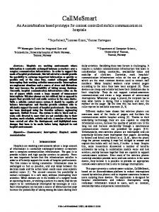
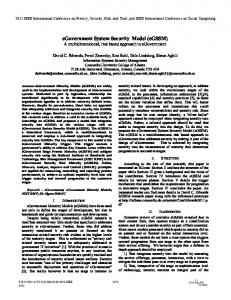
This section illustrates how the Lagrange computer program might be utilized to investigate computer hardware design alternatives. Although the results in this paper are applicable to all closed queuing networks which satisfy the problem formulation, the examples will be limited to central server models." The central server model is shown in Figure 1 with node 0 as the CPU and m( =3) 1/0 devices. After completing a CPU burst, the program will next require service from I/O device i with probability Pi (i = 1,2, ... , mi), or will complete execution with probabilitypo. Thepi's are called branching probabilities and m

i=o

s0 i, 0

i=O

Pi= 1

The branching probabilities are easily related to the visit counts by Vi = Pi /po (i = 1,2, .. ,m) and VO = 49

llpo. We assume that upon completion of one program, another (statistically identical) program enters the system instantaneously along the new program path. Example 1 consists of a CPU and three I/O devices where the first I/O device is a drum and the other two I/O devices are moving-head disks. The input workload parameters and the component power-function cost estimates associated with Example 1 are given

Figure 1. Central server model with three 110 devices.

Table 1. Workload parameters and device cost estimates for Example 1. Memory cost = $50,000 x (degree of multiprogramming) Cost devicei = cibqiI DEVICE

CPU DRUM DISK 1 DISK 2

BRANCHING PROBABILITY 0.05 0.50 0.30 0.15

W/V *

ai

c;

COST COEFFICIENT** EXPONENT $ 1,147,835.00 0.020 0.55309 0.001 1.00000 11,461,312.00 0.001 5,661,184.00 0.67290 0.001 5,661,184.00 0.67290 i

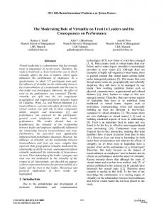
in Table 1. The cost coefficients and power-function exponents come from a small cost-analysis study of IBM 360/370 machines and associated peripherals.'7 With the memory cost function M(n) = $50,000 * n and a budget of $500,000, the optimal device speeds which yield the best throughput are shown in Table 2. A comparison of the optimal throughputs indicates that n = 2 is the best choice for the degree of multiprogramming in Example 1. The parameters which are input to the Lagrange program are designed to capture the needs of the installation being modeled. Unfortunately, the designer may lack sufficient data to accurately characterize these parameters. Since the Lagrange program is inexpensive compared to a simulation program, it can be used effectively to study the sensitivity of system performance to parameter variations. First we study the sensitivity of the results of the optimization when the specified budget is varied. Figure 2 is a graph of optimum throughput as a function of budgetary cost using the same parameters as in Example 1. The optimum throughput was chosen by solving five distinct design problems (n varying from 1 to 5) and selecting the solution with the highest throughput. The curve is divided into four distinct regions and represents an envelope of optimum solutions. In the first region, monoprogramming (n = 1) produces the highest throughput, while in subsequent regions n = 2, 3, and 4, respectively, produce the best predicted throughput. Hence the final output of the Lagrange program provides the optimal integral degree of multiprogramming, the optimal device speeds, and the optimal throughput for each

* WO/ VO = the average number of instructions (in millions) per CPU visit; Wj/V, (i = 1,2,3) = the number of words (in millions) transferred per I/O transaction. **These coefficients result from assuming a device capacity of 8 million words (drum) and 80 million words (disk).

Table 2. Output from Lagrange program, Example 1. Total budget = $500,000

DEGREE OF MULTIPROGRAMMING 1 2 3 4 5

OPTIMAL

THROUGHPUT* 0.071787 0.091731 0.090190 0.078806

0.063084

DEVICE SPEEDS** CPU 0.0613 0.0560 0.0479 0.0382 0.0296

DRUM DISK 1 DISK 2 0.0042 0.0021 0.0013 0.0032 0.0025 0.0019 0.0014

0.0016 0.0012 0.0009 0.0006

0.0010 0.0007 0.0005 0.0003

*Throughput measured in jobs completed per second. *CPU speed in millions of instructions per second; I/O device speed in millions of words transferred per second (the effects of seek time, latency time, and transfer time are inciuded for a block size of 1000 words). 50

.Figure 2. Sensitivity Analysis l: optimal throughput budget.

vs.

COMPUTER

value of the system budget. It should be noted that this curve gives the global solutions for both Problems I and II. The data points which result in Figure 2 were evaluated using a stepwise regression program to determine an overall power-function fit for system cost as a function of system throughput. With 99.5 percent of the variation explained, the regression analysis resulted in the following fit:

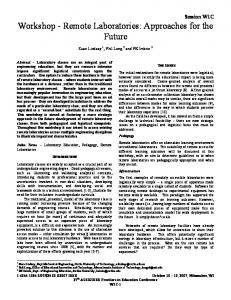
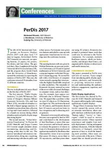
COST = $1,556,605 * T0O4712 This agrees with Grosch's law,15 which states that computing power is proportional to the square of its cost. Figure 3 shows how the money should be allocated among system resources as the budget is varied from $200,000 up to $4,800,000 for Example 1. The optimum throughput was computed for each budget with n varying from 1 to 15. Selecting the best choice of n for a given budget, the cumulative percentages of Figure 3. Sensitivity Analysis II: percent of budget allocated to various the budget which are needed for the hardware compo- devices. Table 3. nents are plotted as a function of the budget in Figure Workload parameters and device cost estimates for Example 2. 3. The bottom curve is the percentage which should Total budget = $500,000 be invested in the CPU. The next curve includes the Memory cost = $50,000 x (degree of multiprogramming) CPU and the drum. The third curve adds on the cost of disk 1, and the top curve results from including the COST COST DEVICE BRANCHING W/V* ' PROBABILITY COEFFICIENT* EXPONENT main memory cost. Although the optimal degree of multiprogramming increases with the total budget CPU 0.05 0.020 $ 1,147,835.00 0.55309 (see Figure 2), the percentage of total budget alDRUM VARIED 0.001 11,461,312.00 1.00000 located to main memory decreases in Figure 3. For DISK 1 VARIED 0.001 5,661,184.00 0.67290 larger installations, the cost of the I/O devices apDISK 2 pears to dominate the budget. 0.10 0.001 5,661,184.00 0.67290 The next sensitivity study relates the change in op- See Table 1 for an explanation of parameters. timal solution to the changes in the branching probabilities (or equivalently, changes in the visit ratios). Table 3 provides the input parameters for this example. Figure 4 shows how optimum throughput changes as the branching probabilities are varied. While Pi is increased from 0.05 to 0.845,p2 is correspondingly decreased such that the sum of all probabilities remains at one. Each curve in Figure 4 represents a different value of the degree of multiprogramming. Note that the optimal degree of multiprogramming remains at two for the entire range of branching probability changes.

Heuristic solution techniques The Lagrange technique discussed so far provides an efficient tool for system design. However, it requires the solution of the system of nonlinear equations. Simpler heuristic techniques may be helpful to a designer who does not require an exact optimization. Besides requiring very little computation, heuristic techniques sometimes require fewer input parameters. This may be important since the input parameters (both workload and cost) are rarely known accurately. Two heuristic solution methods will be discussed and their results will be compared with the exact (Lagrange) technique. April 1980

Figure 4. Sensitivity Analysis Ill: the variation in optimal throughput with branching probability. 51

The first approach to the development of a heuristic technique is to simplify the system of equations (7) by making assumptions on the input parameters. If the assunmptions are not satisfied then the technique can still be used as a heuristic. If we assume that cost exponents are equal, that is, if a0 = = am, the S0 term drops out of Equation (7a) a, and the optimal r8's can be determined independent of the cost equation, (7b). Additionally, ifD1 = ... = Din, then it can be shown that the optimal relative utilizations satisfy the relation, r; = r= ... = r. This assumption used by Ferrari (problem 8.1)3 reduces the problem to a single equation (7a) plus the cost equation (7b). Alternatively, if D1 = D2 . . = Dm = 1, then the optimal relative utilizations satisfy the condition, r = = ... = rm =1 =ro. Thus the relative (and hence, the real) utilizations of all devices will be identical in this case. The system is then said to be load-balanced. The cost equation (7b) is easily solved for the only remaining variable, So, and Si is obtained from Si = (V0 S0)/ Vi. Finally, the speed of device i is obtained using Equation (1). It should be noted that this technique of load balancing will produce the optimal solution only when the assumptions (D1=D2... =D =landai=a2l=am)are satisfied. If these assumptions are not satisfied, then the technique is simply a heuristic for solving the configuration design problem. Our next approach to the derivation pf a heuristic technique is to simplify the system of equations and consider thp case when the number of I/O devices m = 1 and cost exponents a0 = a1. Equation (7a) then reduces to + (+{nnn+1)D + 1)DI r,n+l+l DI r,2n+l+al

-nrl+l + nDir,

+ (n+1)r W

1

(8)

=0

IfD1 = 1, r, = 1 isanexact solution. If D1 > 1 and the first and third terms domir ate Equation (8). Ignoring the other terms results in the ap-

Table 4. Comparison of heuristics with Lagrange method for the central server model.

TH ROUGHPUT* BUDGET $ 100,000

500,000 750,000 920,000 1,250,000 2,000,000 2,500,000

3,500,pOO

4,000,000

5,aoo,000

OPTIMAL DEGREE OF

COST

LOAD

(EXACT

1 2 3 4 5 6 7 9 10

0.002 0.091 0.208 0.310

0.001 0.078

0.002 0.092 0.212 0.317 0.574 1.378 2.059 3.710 4.659

BALANCING BALANCING LAGRAN(GE. MULTIPROGRAMMING HEURISTIC HEURISTIC METHOI

12

*Throughput measured in jobs per second. 52

0.557

1.322 1.965 3.512 4.339

6.364

0.189

0.290 0.537 1.320 1.990 3.613

4.549

6.631

-6.765

proximation n+al

n

Similarly, when D1 >> 1, r«l

(nD

Once the relative utilizations are chosen, the corresponding value for S0 can be obtained by substituting (9) into the cost equation (7b) and solving for So using the ZSYST1M subroutine of the IMSL library. Unlike the load-balancing technique, this technique selects different relative utilizations depending on the value of D , which in turn depends upon the relative costs of the CPU and the I/O device. Thus, a costlier device (with C'i > C0 implyingDi < 1) will be overloaded (that is, ri > 1) and a cheaper device will be underloaded (that is, ri < 1). For this reason, we call this technique the cost-balancing heuristic. Table 4 compares the throughputs resulting from using these two heuristic techniques with the optimal solutions obtained from the exact (Lagrange) technique as the total budget is varied from $100,000 to $5,000,000. The load-balancing heuristic gives poor answers for low budgets, but the answers improve with increasing budgets. The cost-balancing heuristic gives exact answers for low budgets and continues to give nearoptimal results for higher values of the budget. This behavior can be explained as follows. From Figure 2, it is clear that the optimal degree of multiprogramming, n*, increases monotonically with the budget. For higher budgets, n* will be large and the load-balancing heuristic produces a good approximation to the system with optimal throughput due to Theorem 3, which states that as the optimal degree of multiprogramming increases, the optimal relative utilizations approach unity. With a low budget, monoprogramming is optimal and the cost-balancing heuristic tends to give better answers. This can be explained as follows. In the monoprogramming case (n 1), Equation (9) reduces to I1 r.=-

1

+ai

(10) COMPUTER

By direct substitution into Equation (7a), this can be shown to be the exact solution in the monoprogramming situation when ao = ai. With an appropriate change of notation, Equation (10) reduces to the memory balance theorem given by Welch.22 Thus, the cost-balancing heuristic is an extension of Welch's result to the multiprogramming case. Although not optimal, in the general case, the ri values specified by Equation (9) provide a heuristic which produces nearoptimal system design.

The introduction of these two heuristics may be helpful to the user who does not require an exact optimization. By employing both heuristics, the designer can simply select the heuristic solution with better throughput. This implies that the designer need not know whether the budget is low or high compared to the component costs. Our experience indicates that the combined use of the two heuristics yields a nearoptimal design over a wide budget range.

Conclusion Modeling computer systems with a closed queueing network enables selecting the device speeds and main memory size that will maximize throughput or minimize costs. System component costs are approximated by continuous power-function estimates of cost in terms of device speeds. Using the Lagrangian method the configuration design problem is converted into a system of nonlinear equations. If the system designer can adequately characterize system workload and requires optimal computer component speeds, the Lagrange multiplier program is an efficient tool. Alternatively, the load-balancing heuristic and cost-balancing heuristic can provide fairly good rules of thumb. Several extensions to the model have been carried out. First, we have developed a design model of a multiprogramming system with paging.23 Secondly, the design model of the present paper assumes that the branching probabilities (pi's) in the central server model are fixed input parameters, but they would vary with the assignment of files to secondary storage devices in a real system. Combining the file assignment problem with the hardware selection problemis the subject of another paper.24 Finally, a design model of linear storage hierarchies is discussed in Reference 25. R

Acknowledgments Thanks are due to Dr. John Spragins, Dr. T. M. Sigmon, Dr. R. A. Wagner, J. G. Rusnak, and the referees for their useful comments. Dr. M. Phister suggested that the parameterization of the examples be modified from the data in Reference 17 to make the problems more realistic. This work was supported in part under National Science Foundation grant US NSF MCS 78-22327 and National Library of Medicine grants LM-003373 and LM-07-003.

References 1. K. M. Chandy and R. T. Yeh, eds., Current Trends in Programming Methodology, Vol. III: Software Modeling, Prentice-Hall, Englewood Cliffs, N. J., 1978. 2. P. J. Denning and J. P. Buzen, "The Operational Analysis of Queueing Network Models," Computing Surveys, Vol. 10, No. 3, Sept. 1978, pp. 225-261. April 1980

53

3. D. Ferrari, Computer Systems Performance Evaluation, Prentice-Hall, Englewood Cliffs, N. J., 1978. 4. L. Kleinrock, Queueing Systems-Vol. 2: Computer Applications, Wiley, New York, 1976. 5. K. S. Trivedi, "Analytic Modeling of Computer Systems," Computer, Vol. 11, No. 10, Oct. 1978, pp. 38-56. 6. F. Baskett, K. M. Chandy, R. R. Muntz, and F. G. Palacios, "Open, Closed, and Mixed Networks of Queues with Differrent Classes of Customers,"JACM Vol. 22, No. 2, Apr. 1975, pp. 248-260. 7. W. W. Y. Chiu, "Analysis and Applications of Probabilistic Models of Multiprogrammed Computer Systems," PhD dissertation, Department of Electrical Engineering, University of California, Santa Barbara, Calif., Dec. 1973. 8. S. K. Kachhal and S. R. Arora, "Seeking Configurational Optimization in Computer Systems," Proc. ACMAnn. Conf., 1975, pp. 96-101. 9. K. S. Trivedi and R. A. Wagner, "A Decision Model for Closed Queueing Networks," IEEE Trans. Software Eng., SE-5, No. 4, July 1979, pp. 328-332. 10. K. M. Chandy, J. H. Howard, Jr., and D. F. Towsley, "Product Form and Local Balance in Queueing Networks," JACM, Vol. 24, No. 2, Apr. 1977, pp. 250-263. 11. J. P. Buzen, "Queueing Network Models of Multiprogramming," PhD thesis, Division of Engineering and Applied Physics, Harvard University, Cambridge, Mass., May 1971. 12. A. C. Wiliams and R. A. Bhandiwad, "A Generating Function Approach to Queueing Network Analysis of Multiprogrammed Computers," Networks, Vol. 6, No. 1, Jan. 1976, pp. 1-22.

I

SOFTWARE ENGINEERS

THINK PARALLEL

13. IMSL Reference Manual, IMSL, Inc., Houston, Tex., 1979. 14. K. M. Chandy, J. Hogarth, and C. H. Sauer, "Selecting Capacities in Computer Communications Systems," IEEE Trans. Software Eng., SE-3, No. 4, July 1977, pp. 290-295. 15. M. Phister, Data Processing Technology and Economics, Santa Monica Publishing Co., Santa Monica, Calif., 1976. 16. D. G. Luenberger, Introduction to Linear and Nonlinear Programming, Addison-Wesley, Reading, Mass., 1973. 17. R. E. Kinicki, "Queueing Models for Computer Configuration Planning," PhD dissertation, Department of Computer Science, Duke University, Durham,,N.C., 1978. 18. J. P. Buzen, "C6mputational Algorithms for Closed Queueing Networks with Exponential Servers," CACM, Vol. 16, No. 9, Sept. 1973, pp. 527-531. 19. F. R. Moore, "Computational Model of a Closed Queueing Network with Exponential Servers," IBM JRD, Vol. 16, No. 6, Nov. 1972, pp. 567-572. 20. K. M. Brown, "A Quadratically Convergent Newtonlike Method Based upon Gaussian Elimination," SIAM J. Numer. AnaL, Vol. 6, No. 4, Dec. 1969, pp. 560-569. 21. P. J. Denning, K. C. Kahn, J. Leroudier, D. Potier, and R. Suri, "Optimal Multiprogramming," Acta Informatica, Vol. 7, No. 2, 1976, pp. 197-216. 22. T. A. Welch, "Memory Hierarchy Configuration Analysis," IEEE Trans. Computers, Vol. C-27, No. 5, May 1978, pp. 408-413. 23. K. S. Trivedi and T. M. Sigmon, "A Performance Comparison of Optimally Designed Computer Systems with and without Virtual Memory," Proc. 6th Annual Int'l Symp. on Computer Architecture, Apr. 1979, pp. 117-121. 24. K. S. Trivedi, R. A. Wagner, and T. M. Sigmon, "Optimal Selection of CPU Speed, Device Capacities and File Assignments," to appear in J. ACM. 25. K. S. Trivedi and T. M. Sigmon, "Optimal Design of Linear Storage Hierarchies," to appear in J. ACM

Goodyear Aerospace Corporation is the world leader in parallel computing. If you would like to step up from sequential to parallel processing contact us.

Kishor S. Trivedi is an associate professor of computer science at Duke University in Durham, North Carolina. His current research interests include com-

GAC markets the STARAN parallel computer. We have developed a Micro Array Multi-Proc-

essor. We are currently developing a Massively Parallel Processor for NASA.

Goodyear needs experienced software engineers to develop system and application software for computers. Sequential experience is just fine. We will teach you all you need to know about parallel computing. Send resume and salary requirements to: E.L. Searle, Personnel Goodyear Aerospace Corporation Akron, Ohio 44315 An Equal Opportunity Employer

A * E >

puter architecture, performance-oriented design of computer systems, and fault-tolerant computing. A distin-

guished visitor of the IEEE Computer Society since 1976, Trivedi received the w B. Tech degree in electrical engineering

V

from the Indian Institute of Technology, Bombay, India, and the PhD degree in computer science from the University of Illinois, Urbana, in 1968 and 1974, respectively.

Robert E. Kinicki is an assistant professor in the Computer Science Department at Worcester Polytechnic Institute in Worcester, Massachusetts. He teaches courses in operating systems and performance evaluation and is currently doing research in the area of medical computer applications at the University of Massachusetts Medical -;' 0Center. He received the MS degree in computer science from Indiana University in 1975 and the PhD degree from Duke University in 1978.

X

COMPUTER