A modem regression approach to determining fault ... - Science Direct

Journalof StructuralGeology,Vol. 18, Nos 2/3, pp. 147 to 152, 1996 Copyright © 1996 Elsevier Science Ltd Printed in Great Britain. All rights reserved 0191-8141/96 $15.00+ 0.00

Pergamon

01914141(96)00110-7

A modem regression approach to determining fault displacement4ength scaling relationships R. M. CLARK Department of Mathematics, Monash University, Clayton, Victoria 3168, Australia

and S. J. D. COX Australian Geodynamics Cooperative Research Centre, CSIRO Exploration and Mining, PO Box 437, Nedlands, WA 6009, Australia

(Received 21 April 1995; accepted in revisedform 29 August 1995) Abstract--A number of studies have supported the hypothesis that fault displacement is systematically related to fault size by a power law. The relationship is important for estimating bulk strain in faulted terrains. However, the exponent of this relation has been the subject of some dispute: in particular as to whether the exponent is unity (i.e. a linear relationship exists between displacement and length) or larger. The techniques used to determine the exponent have been inconsistent and far from rigorous in their application of statistical tests and terminology. We have re-analysed several of the data sets using more careful techniques. We find that the power law with an exponent of unity explains most sets of data when analysed separately. We also applied a weighted joint regression analysis to combined data covering nearly 6 orders of magnitude. The best estimate of the common slope (slope in log-log space = exponent of a power law in linear space) is 0.946 with a standard error of 0.0426. Statistical tests confirm that this exponent is consistent with a value of unity, implying a linear relationship between fault displacement and length within each data set. However, the different data sets have varying intercepts in the log-log space, indicating differing slopes for the linear relation.

In this study we use modern regression techniques to re-examine the evidence for and against such a relationship. We use 11 data sets used in previous analyses. In particular, we investigate whether or not a common value of c applies for all 11 data sets, and if so, whether this common c is consistent with any of the competing hypotheses. We assume that, given a fault of length L, the corresponding observed maximum displacement D is given by the equation

INTRODUCTION It has been suggested that the relationship between displacement D and length L in a population of bounded faults in continental areas is of the form O -

Lc

P

(1)

apart from random noise in the measurements of D andIor L, where c and P are constants for a particular data set. This may also be written logD= K+ clogL, K=-logP.

logD= K+clogL

(2)

The relationship is important, since when combined with a frequency-length relation, it allows an estimate of the total strain in a region of faulted rock using a sampling of fault sizes (Scholz & Cowie 1990, Marrett & Allmendinger 1991, 1992, Walsh et al. 1991, Walsh & Watterson 1992). Furthermore, it provides primary evidence regarding the mechanics of fault initiation and growth (Watterson 1986, Cowie & Scholz 1992a, Burgmann et al. 1994). Previous studies have generally accepted the powerlaw hypothesis and have focused on determining the parameters of the power law. It has been proposed that a common exponent c, at least, may apply, but various values have been suggested, e.g. c = 1.0 (Cowie & Scholz 1992b), c = 1.5 (Marrett & Allmendinger 1991) or c = 2.0 (Watterson 1986, Walsh & Watterson 1988).

+e,

(3)

where e denotes a random error. In the population of faults, the random error e is assumed to have an average value of zero, Each individual error derives from two components: (i) the 'pure-error' or 'within-fault' variability which relates to the sampling technique, and is exemplified by fig. 2 of Cowie & Scholz (1992b); and (ii) a lack-of-fit component, which recognizes that equations (1) and (2) are only idealized formulae. These two components of variability can be estimated from those instances of multiple Ds for the same L. In the model expressed by equation (3) the random error in the data is additive on the logarithmic scale, i.e. multiplicative on the original scale. This is a necessary and reasonable assumption; it means that with data covering several orders of magnitude, the random errors remain in the s a m e p r o p o r t i o n , e.g. 100 m in 1 km and 10 cm in 1 m.

147

148

R . M . C L A R K and S. J. D. COX

We make the further assumption that the lengths L of the faults can be determined to a greater accuracy than the measurement of maximum displacement D. This has the important consequence that it is valid, by a conditioning argument (Cox & Hinkley 1974, Chap. 2), to apply standard least-squares regression methods to the estimation of the parameters K and c in equation (3), regardless of how the faults were sampled. The modern regression approach used here has further advantages. It is possible and advisable to group all the data together and estimate the common value of c from these combined data. Various hypotheses of interest can be tested automatically, using standard statistical tests, and the total variability of the data can be partitioned up into various components of interest. Finally, all the assumptions of the model can be tested.

DETAILS OF THE ANALYSIS We performed the analysis on 11 data sets consisting of: (i) eight of the sets used by Cowie & Scholz (1992b), excluding the MacMillan data (for the reasons discussed by them); and (ii) three additional sets digitized from fig. 2 of Watterson (1986). The original sources are indicated in Table 1. We used the statistical computing package M I N I T A B (Release 7.2, Minitab Statistical Software, 3081 Enterprise Drive, State College, P A 16801-2756, U.S.A.) for all the numerical analyses. One-at-a-time With 11 groups of data (see Table 1) we use a more general version of equation (3), namely log Dij = Ki + c~ log Lij + eli,

(4)

where (Dip Lij) represents thej-th pair of D - L measurements in the i-th group, and K i and ci denote the intercept and slope of the log D - log L line for the i-th group. Within the i-th group, the error terms e;j are assumed to follow a Normal or Gaussian distribution with a standard deviation cry. The assumption of normality is not critical, and will be tested anyway.

The 11 separate regression lines specified by the model described by equation (4) were fitted one-at-atime, yielding results shown in Table 1. In nine of the 11 groups, the estimated slope di was consistent with Cowie & Scholz's (1992b) hypothesis of c = 1 as judged by the standard t-statistic which counts how many standard errors the estimate is from the hypothesis. A value of t between - 2 and +2 means that there is no statistical evidence against the hypothesis that c = 1, at the 5% significance level. The t-test automatically takes account of the relatively small number of observations within each group, the scatter about the fitted line, and the possibly unequal spacing of the log Ls within the group, The experimental lack-of-fit test (XLOF) (Burn & Ryan 1983) in M I N I T A B also showed that within each group there was no significant nonlinearity in the plot of log D against log L (Clark & Cox 1995). Some faults in group 8 (Walsh & Watterson 1987) contained measurements across multiple profiles. An analysis of these repeated measurements showed that within-fault variation of the D - L relationship is not as serious a problem as fig. 2 of Cowie & Scholz (1992b) might suggest. In addition the related 'pure-error' lackof-fit test confirmed that the assumption of a linear model (3) was satisfactory (Clark & Cox 1995). Cowie & Scholz (1992a) suggest that c = I is consistent with control of fault formation by a fracture mechanics mechanism with residual friction. Those data which do not have c -- 1 may be controlled by qualitatively different mechanics. For example, the Opheim & Gudmundsson (1989) data are from surface fractures in lava flows in Iceland, so these may have been influenced by thermal shrinkage, causing a deviation from the elastic relation. The residual standard deviations (Oi in column 7 of Table 1) are clearly very different, as confirmed by Bartlett's test (Bartlett 1937) yielding a highly significant T = 41.5 on 10 degrees of freedom (d.f.). There was no clear pattern in these residual standard deviations, as a function of either fault type or mean fault length. Any further statistical analysis based on the combined data will therefore need to take account of this heterogeneity of variance by appropriate weighting.

Table 1. Summaryof one-at-a-timeanalyses---11groups, n = number of faults, di = estimate of power-lawexponent c, SE(d/) = standard error of this estimate, t = standard t-statistic with respect to hypothesisthat c = 1, Oi= residual standard deviationof the samples around the best-fit line and W = weight factor used in the subsequent combinedanalysis i

Source

n

~i

SE((~i)

t

Oi

W

1 2 3 4 5 6 7 8 9 10 11

Elliott (1976) Krantz (1988) Muraoka& Kamata (1983) Opheim & Gudmundsson (1989) Peacock (1991) Peacock & Sanderson (1991) Villeminet al. (1995) Walsh & Watterson (1987) North Derby (Watterson 1986) Barnsley (Watterson 1986) Mid-ocean(Watterson 1986)

29 16 15 7 20 20 26 34 18 18 7

1.0143 1.4439

0.08452 0.2270 0.1915 0.0628 0.0999 0.2024 0.0643 0.2144 0.2082 0.1640 0.1299

0.17 1.96 -0.49 -5.31 -6.15 -0.88 -1.94 0.39 -1.78 -0.99 0.99

0.1763 0.2776 0.2217 0.0532 0.1775 0.3224 0.1735 0.3480 0.2542 0.1685 0.1410

0.175 0.250 0.250 --0.330 0.175 0.330 0.250 0.175 0.175

0.9058

0.6666 0.3850 0.8209 0.875

1.0846 0.6287 0.8280 1.1290

Statistics of fault displacement-length relations

2

I

I

I

I

149

I

I



1

x

2

o ÷

6 7

A

8

*

9

n

10

1 ~

+

11

-1 + i0

8 E

-2

Q.

._m '1o

_g

-3 9 E]

[] D / s -4

in

-5 3/4.

-6 ..g

n I

I

I

I

I

I

-3

-2

-1

0

1

2

3

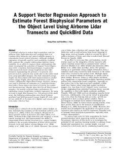
log length (km) Fig. 1. Results of the combined analysis of nine data sets (lines), with the source data (symbols). Group numbers as in Table 1. Table 2. Analysis of variance for combined weighted regressions

Source of variation Regression Differences between intercepts (assuming common slope) Residual error: Differences between slopes Lack of fit to parallel lines Pure error (within faults) Total

Degrees of freedom

Sum of squares

(d.f.)

(S.S.)

1 8 173 8 148 17 182

Combined analysis Clearly, the estimates of c in groups 4 and 5 are different from all the rest. We now use m o d e m regression analysis to consider whether the combined data in the remaining nine groups are consistent with a common value of c (parallel lines across groups), or even a common K as well (a single line for all groups). In weighted regression analysis we pool the nine groups into a super-group of 183 observations while still allowing the subsets to have different scaling factors P and different within-group precision. This is achieved as follows. The data sets are assigned to three groups on the basis of their residual standard deviations, and each of

9354.3 577.6 178.65 12.76 152.34 13.55 10,110.5

Mean square = S.S./ d.f. (M.S.) 72.2 1.03266 1.595 1.029 0.797

the subsets weighted as shown in the last column of Table 1, based on the corresponding average residual standard deviations. This implicitly rescales all the data so that the subsequent analysis becomes essentially scale-free. With this rescaling, the residual standard deviation for any satisfactory model should be close to unity. Weighted least-squares regression was used to fit: (i) nine parallel lines (with different intercepts in each group---Fig. 1); and (ii) a single line to the combined data from all groups. The results of our combined analysis are summarized in the conventional 'analysis of variance' table (Table 2). This enables various hypothesis of interest to be tested

150

R . M . CLARK and S. J. D. COX Table 3. Estimates of intercepts under parallel-line m e t h o d (see Table 1 for sources of data), n = n u m b e r of faults in group, /~ = estimate of intercept in log-log space, SE(/~) = standard error of estimate, P = estimate of scaling factor in power law (P = 10r), PL and P u = lower and upper 95% confidence bounds on the estimate, P* = estimate of scaling factor derived from Cowie & Scholz (1992b) where P = 1/y i

n

/~

SE(/~)

P

1 2 3 6 7 8 9 10 11

29 16 15 20 26 34 18 18 7

- 1.1074 -2.2983 -2.100 -2.1972 - 1.4730 -2.3235 -2.5569 -1.9825 -2.0332

0.0837 0.0638 0.1424 0.1237 0.0389 0.0576 0.0600 0.0423 0.0807

12.11 198 126 157 30 211 360 96 108

PL

Pu

P*

7.1 148 65 89 25 162 273 79 74

15.3 267 243 278 35 275 475 117 157

16.7 143 83.3 111 34.5 166.7 ----

Note: 95% confidence limits = 10 (r±2°sE). Formal significance test for differences between the estimated Ks should take account of the correlations between these estimates. (See Clark & Cox 1995 for details.)

simply by comparing the mean squares (last column). The lower part of the table confirms that each data set is close to a straight line in log-log space. In the top part, the very large mean square of 72.2 show that the combined data are not consistent with a single-line fit across all groups, in contrast to Watterson (1986) and Marrett & Allmendinger (1991). However, the data are quite consistent with the hypothesis of parallel lines with a common slope for nine of the 11 groups. See Clark & Cox (1995) for further discussion and formal significance tests. The best (unbiased) estimate of this common slope is = 0.946, with a standard error of 0.0426. This estimate of the exponent c is clearly consistent with Cowie & Scholz's (1992b) hypothesis that c = 1 (t = -1.34), and is inconsistent with the alternative hypotheses that c = 1.5 (t -- 13.0) (Marrett & Allmendinger 1991) and c = 2 (t -- 24.7) (Watterson 1986, Walsh & Watterson 1988). The analysis also produced estimates of the scaling factor P in equation (1) together with approximate 95% confidence limits (Table 3). We found that these estimates varied widely, which would be consistent with the different data sets involving different materials and geological histories. However, the sets covering larger faults tend to have lower values of P (Elliott 1976, Villemin et al. 1995) consistent with the observed tendency between data sets which has previously led to the grouping of all the data around a single line with a slope greater than unity (Walsh & Watterson 1988, Marrett & Allmendinger 1991). This is an important observation, though the explanation is not clear. As noted by Cowie & Scholz (1992b) it is at least probable that there will be a consistent change when the faults become so large that they are no longer bounded in three dimensions within their host brittle layer (e.g. Pacheco & Scholz 1992, Davy 1993, Westaway 1994). In Table 3 we also show P* which is the reciprocal of ~(= 1/P for c -- 1) from Cowie & Scholz's (1992b) table 1 for comparison. In most cases these fall within the bounds suggested by our analysis.

TESTING ASSUMPTIONS Binning

If the measurement of either L or D is subject to rounding, which is common particularly if the variables are determined by conversion of seismic magnitudes, then the data may be considered to be grouped or 'binned'. This can have an effect on parameter estimation (Fryer & Pethybridge 1972). Here binning does not appear to be severe, so we have not applied any correction. Measurement errors

However, the lengths of faults are probably subject to errors of measurements of the order of 10-20%. We tested the effect of this on the analysis empirically. We added random Gaussian noise to the log-lengths, with standard deviation 0.04 (i.e. log 1.1) which is equivalent to working with data in which roughly a third of the lengths would be in error by at least 10%. A repeat of the entire regression analysis with these jittered lengths produced exactly the same conclusions as the first analysis, with only minor changes to estimated parameters. Our results and conclusions appear to be robust under fairly realistic imprecision in the lengths. Error distribution

We tested the distribution of the random errors e using normal quantile plots (Filliben 1975) and found the assumption that they are Gaussian-distributed is reasonable. We also found random scatter in residual plots, confirming that the parallel lines model is a good fit to the data (Clark & Cox 1995). Our assumptions regarding the random errors e in equations (3) and (4) are not critical however, since the t-values for c are so clear-cut. The conclusions, both

Statistics of fault displacement-length relations qualitative and quantitative, appear to be insensitive to moderate levels of inaccuracy in the lengths.

NOTES ON REGRESSION ANALYSIS AND STATISTICAL TOOLS

Correlation coefficient Some authors use the correlation between log D and log L, as measured by the least-squares correlation coefficient, r, to indicate the reliability of their estimate of c. This is incorrect, since although the correlation coefficient measures how close the data are to a straight line, it says nothing about the slope of that line. In particular, the correlation coefficient may fail to indicate systematic variations from linearity. That is much better tested by examining the residuals for a systematic pattern, or by methods such as the XLOF test used here (Clark & Cox 1995). In particular, an undetected nonlinearity makes extrapolation of the relation to estimate derived parameters, such as bulk strain, very dangerous. Formal tests of significance for the correlation coefficient are available only for Gaussian distributions. Thus, even though it is possible to compute a correlation coefficient for an arbitrary data set, even a high value may be misleading and give a false sense of confidence.

Effect of sample distribution on parameter estimates Cowie & Scholz (1992b), note that within a given region, the lengths L of faults may follow a power-law distribution, with many small faults but relatively few large ones. They suggest that this over-representation of small faults renders 'a fit to the data statistically biased'. This is incorrect since this least-squares analysis is conditional on the Ls actually observed. Provided only that the random errors e in (3) and (4) have zero mean, then the least-squares estimates of all the cs and Ks are not biased (Kendall & Stuart 1973, section 28.14). However, the precision of these least-squares estimates does depend on the configuration of the Ls in the actual sample. In general, the least-squares estimates become less precise as the distribution of the log-lengths becomes more skewed (Clark & Cox 1995). Fortunately, the configuration in our combined data is almost uniform, due to combining data-sets each covering only a part of the total range of the Ls. Cowie & Scholz (1992b) also suggest that "each data set spans . . . too short a range" to give a reliable estimate of the exponent c. While the standard error of from any small data set could be high in absolute terms, such an estimate is always unbiased, and in most cases the estimate of the slope is more accurate than the original measurements (Clark & Cox 1995). In any case, by fitting parallel lines to the combined data, our analysis utilizes 183 lengths and displacements, ranging over 6 orders of magnitude, to reliably estimate the exponent c.

151

Testing the hypotheses Finally, while intuitively appealing, the method used by Cowie & Scholz (1992b) to test the competing hypotheses c = 1.0 and c = 1.5 (see their table 1) has significant flaws. First, it takes no account of the differing sample sizes, or of the random noise in the data. Also, since the P-values for c = 1.5 in their table 1 are not actually estimated from the D - L data, the increase in variance which they found might be due to having the wrong value of P. Both of these objections are overcome by the straightforward t-tests used in our analysis. CONCLUSIONS We have considered the problem of whether fault displacements and lengths are related by a power law, and what the value of the power-law exponent is. Our study applied modern regression techniques to perform a rigorous statistical analysis. We examined the same data as earlier studies, which have been the basis of a dispute about the values of the parameters in the power law, in particular whether the power-law exponent is unity or larger. We find that most of the data examined are consistent with a linear relationship (a power-law exponent of unity) between fault displacement and length, and that exponents of 1.5 or 2 are clearly inconsistent with the data. The results are robust, being based on methods which use all of the data simultaneously, covering nearly 6 orders of magnitude in fault length as well as a separate analysis of the individual data sets, and are also not affected by the likely imprecision in the original measurements. Furthermore, the analysis is not dependent on, or biased by, the underlying distribution of fault sizes. Individual data sets may have different intercepts in log-log space (corresponding with different slopes for the linear relation) and there is a tendency for larger faults to have even larger displacements. However, this effect is not systematic. The statistical treatment presented here, part of which considered the combined data in a way that does not assume that the data need be homogeneous, clearly demonstrates that a unity exponent (i.e. a linear relation) is most appropriate for individual data sets, although the scaling factors differ between the data sets, so no single linear relationship is consistent with all data.

Acknowledgements--We would like to thank Patience Cowie and John Walsh for kindly sending us copies of their data. Comments by Bill Power, and reviews by Nancye Dawers, Patience Cowie and Steven Wojtal helped improve the presentation. This work was largely completed during a study-leave visit by RMC to CSIRO in JanuaryFebruary 1995. Other support was provided by ARC grant A39031709 and the Australian Geodynamics Cooperative Research Centre.

REFERENCES

Bartlett, M. S. I937. Properties of sufficiencyand statistical tests. Proc. R. Soc. Lond. AI60, 268-282.

152

R . M . CLARK and S. J. D. COX

Burgmann, R., Pollard, D. D. & Martel, S. J. 1994. Slip distribution on faults: effects of stress gradients, inelastic deformation, heterogeneous host-rock stiffness, and fault interaction. J. Struct. Geol. 16, 1675-1690. Burn, D. A. & Ryan, T. A. Jr, 1983. A diagnostic test for lack of fit in regression models. Am. Stat. Assn Proc. of Statistical Computing Section, 286--290. Clark, R. M. & Cox, S. J. D. 1995. Statistical analysis of fault lengths and displacements. CSIRO Expl. & Min. Open-file Rep. 140F. Cowie, P. A. & Sehoiz, C. H. 1992a. Physical explanation for the displacement-length relationship of faults using a post-yield fracture mechanics model. J. Struct. Geol. 14, 1133-1148. Cowie, P. A. & Scholz, C. H. 1992b. Displacement-length scaling relationship for faults: data synthesis and discussion. J. Struct. Geol. 14, 1149-1156. Cox, D. R. & Hinkley, D. V. 1974. Theoretical Statistics. Chapman & Hall, London. Davy, P. 1993. On the frequency-length distribution of the San Andreas fault system. J. geophys. Res. 98, 12,141-12,151. Elliott, D. 1976. The energy balance and deformation mechanisms of thrust sheets. Phil. Trans. R. Soc. Lond. A203, 289-312. Filliben, J. J. 1975. The probability plot correlation test for normality. Technometrics 17, 111-117. Fryer, J. G. & Pethybridge, R. J. 1972. Maximum likelihood estimation of a linear regression function with grouped data. Appl. Stat. 21,142-154. Kendall, M. G. & Stuart, A. 1973. Advanced Theory of Statistics, Vol. 2. Griffin, London. Krantz, R. W. 1988. Multiple fault sets and three-dimensional strain: theory and application. J. Struct. Geol. 10, 225-237. Marrett, R. & Allmendinger, R. W. 1991. Estimates of strain due to brittle faulting: sampling of fault populations. J. Struct. Geol. 13, 735-738. Marrett, R. & AIImendinger, R. W. 1992. Amount of extension on "small" faults: an example from the Viking Graben. Geology 20, 4750.

Muraoka, H. & Kamata, H. 1983. Displacement distribution along minor fault traces. J. Struct. Geol. 5, 483--495. Opheim, J. A. & Gudmundsson, A. 1989. Formation and geometry of fractures and related volcanism, of the Krafla fissure swarm, northeast Iceland. Bull. geol. Soc. Am. 101, 1608-1622. Pacheco, J. F. & Scholz, C. H. 1992. Changes in frequency-size relationship from small to large earthquakes. Nature 355, 71-73. Peacock, D. C. P. 1991. Displacement and segment linkage in strikeslip fault zones. J. Struct. Geol. 13, 1025-1035. Peacock, D. C. P. & Sanderson, D. J. 1991. Displacement and segment linkage and relay ramps in normal fault zones. J. Struct. Geol. 13, 721-733. Scholz, C. H. & Cowie, P. A. 1990. Determination of total strain from faulting using slip measurements. Nature 346, 837-839. Villemin, T., Angelier, J. & Sunwoo, C. 1995. Fractal distribution of fault length and offsets: Implications of brittle deformation evaluation - - the Lorraine Coal Basin. In: Fractals in the Earth Sciences (edited by Barton, C. & LaPointe, P.). Plenum Press, New York, 205-226. ' Walsh, J. J. & Watterson, J. 1987. Distribution of cumulative displacement and of seismic slip on a single normal fault surface. J. Struct. Geol. 9, 1039-1046. Walsh, J. J. & Watterson, J. 1988. Analysis of the relationship between displacements and dimensions of faults. J. Struct. Geol. 10, 239-247. Walsh, J. J. & Watterson, J. 1992. Populations of faults and fault displacements and their effects of estimates of fanlt-related regional extension. J. Struct. Geol. 14,701-712. Walsh, J. J., Watterson, J. & Yielding, G. 1991. The importance of small scale faulting in regional extension. Nature 551,391-393. Watterson, J. 1986. Fault dimensions, displacements and growth. Pure & Appl. Geophys. 124, 366-373. Westaway, R. 1994. Quantitative analysis of populations of small faults. J. Struct. Geol. 16, 1259-1273.