coding outweigh the loss in mutual information incurred by the transformation. More specifically, for any network of Gaussian channels for which lattice encoding ...
A Modulo-Lattice Transformation for Multiple-Access Channels Uri Erez† and Ram Zamir∗ Dept. of Electrical Engineering - Systems Tel-Aviv University Tel-Aviv 69978, Israel Email: {uri,zamir}@eng.tau.ac.il Abstract—A simple lemma is derived that allows to transform a general single-user (non-Gaussian, non-additive) continuousalphabet channel as well as a general multiple-access channel into a modulo-additive noise channel. While in general the transformation is information lossy, it allows to leverage linear coding techniques and capacity results derived for networks comprised of additive Gaussian nodes to more general networks. Index Terms—Lattice codes, Network coding , Additive Noise.
I. I NTRODUCTION There has been considerable progress in recent years in deriving structured coding schemes and capacity results for single-user channels as well as networks with AWGN noise, e.g., [2], [7], [10], [4], [6], [1]. A key ingredient in these results is the use of linear/lattice codes that are particularly well suited for additive noise channels. In this work, we derive a lemma that allows to leverage these techniques to networks which have general multiple-access channels (MAC) nodes. Specifically, we provide a transformation that transforms a general (neither Gaussian nor additive) continuous-amplitude MAC, into an modulo-additive one, at the price of some information loss. For some channels, the rate increase offered by lattice coding outweigh the loss in mutual information incurred by the transformation. More specifically, for any network of Gaussian channels for which lattice encoding schemes are exploited to derive an achievable rate region, using the derived lemma, one may obtain an analogous inner bound on the rate region for a network with the same topology but with general channels. The transformation is a simple extension of the mod -Λ transformation derived for single-user channels as given in [2] and specifically the version given by Forney in [3]. II. M ODULO L ATTICE TRANSFORMATION Consider a general multiple-access channel with M users. For simplicity, the derivation below will be written in terms of a two-user (M = 2) MAC. The extension to the general case is straightforward. We thus assume a two-user MAC with inputs X1 , X2 and output Y , with a general transition ∗ †
This work was supported by the ISF under grant # 1259/08. This work was supported by the ISF under grant # 1234/08.
distribution w(Y |X1 , X2 ), where all random variables are realvalued and continuous. Unless stated otherwise we assume that all transmitters as well as the receiver have full channel knowledge. We further assume that the transmitters are subject to an input constraint. In the following the input constraint will be taken to be a power constraint so that the inputs must satisfy E[Xi2 ] ≤ PX,i . We may transform the channel into a mod -Λ MAC as we describe next. Let Λ be a lattice and let V be some fundamental region of Λ. Let vi ∈ V, i = 1, 2, be the information bearing signals of the users. Further, let Ui ∼ Unif(V), i = 1, 2, be independent dithers uniformly distributed over V. We assume that the dither Ui is known to transmitter i as well as to the receiver1. For any scalar function f : R → R, when operating on an ndimensional vector, we define its operation as the cartesian product extension. That is, for x ∈ Rn , f (x) = (f (x1 ), . . . , f (xn )) . With this notation, the transmitters operate as follows. Transmitter i Computes: X′i = [vi + Ui ] mod Λ.
(1)
Sends the preprocessed signal: Xi = fi (X′i ).
(2)
where fi (·) satisfies the power constraint, E[fi (U)2 ] ≤ PX,i .
(3)
X′i
Note that due to the dither, is uniformly distributed over V (see [2], [3]), for any value of vi . Let S = k1 X′1 + k2 X′2 ˆ = g(Y) be an estimator of S where k1 , k2 are integers. Let S from the output Y. Ideally, the criterion for estimation should be that of minimum noise entropy but any other estimator ˆ − S. The may be used. Denote the estimation error by N = S receiver processes the output as follows. Receiver Computes: ˆ − k1 U1 − k2 U2 ] mod Λ Y′ = [S =
[g(Y) − k1 U1 − k2 U2 ] mod Λ.
(4)
1 In practice, a pseudorandom sequence will be used at both transmission ends.
U1 v1
Σ
X′1 mod-Λ
X1
k1 U1 + k2 U2
f1 (·)
ˆ S
Y
X′2
v2 Σ
mod-Λ
=
Σ
mod-Λ
X2
The general mod Λ transformation.
We now observe that the induced channel from v1 , v2 to Y′ is indeed additive modulo Λ. From (4) and using the definition of S we obtain, ˆ + (S − S) − k1 U1 − k2 U2 ] mod Λ Y′ = [S h ˆ + k1 ([v1 + U1 ] mod Λ) + k2 ([v2 + U2 ] mod Λ) = S i − S − k1 U1 − k2 U2 mod Λ ˆ − S)] mod Λ [k1 v1 + k2 v2 + (S
Y′
f2 (·) Fig. 1.
=
g(·)
w(Y |X1 , X2 )
U2
−
(5)
[k1 v1 + k2 v2 + N] mod Λ,
where (5) follows since k1 and k2 are integers. Note that (V1 , V2 , U) ↔ (X1 , X2 ) ↔ Y forms a Markov chain. Since X1 , X2 are independent of V1 , V2 , so is the pair (S, g(Y)) and hence N. We thus obtain the following lemma, Lemma 1: Applying the transmission scheme (2), (4), results in a mod -Λ additive noise channel: Y′ = [k1 v1 + k2 v2 + N] mod Λ (6) ˆ − S is independent of the inputs v1 and v2 . where N = S We note that the lemma generalizes the single-user version of [2] in several ways. First, it applies to any channel, which need not be Gaussian nor additive2, and thus extends results even for a single-user channel. Second, it treats multiple-access channels as well. We further note that while in [3] the optimal estimator turned out to be linear since the channel considered was an AWGN channel, it is apparent that in a more general setting, non-linear estimation is beneficial. We refer to the application of the functions fi (·) at the transmitters (2) as “preprocessing” and to the application of the function g(·) at the receiver (4) as “postprocessing”. Allowing for preprocessing at the transmitters is of great value, as will be seen in the examples below. The ability of the transmitters to choose suitable preprocessing functions of course depends on their having channel knowledge. Furthermore, in general, determination of the optimal preprocessing and postprocessing functions calls for a joint optimization3. We note that pre2 We note that as opposed to the single-user additive Gaussian case, in general there is information loss associated with having the receiver use only Y′ (i.e., it is not a sufficient statistic) rather than (Y′ , U). 3 In a slowly varying environment, for instance, the pre/post processing functions could be performed at the receiver and the determined preprocessing functions would be fed back to the transmitters.
processing was not allowed for in previous works such as [8] where a time-varying channel model was assumed and no channel knowledge was available to the transmitters. Consider now a single user mod Λ channel Y′
= [ki vi + N] mod Λ.
(7)
Note first that since ki is an integer, as long as it is nonzero, it has no effect on the capacity of the channel, which may be achieved by taking the input Vi ∼ Unif(V), a choice that results also in [ki Vi ] mod Λ ∼ Unif(V). We denote the resulting capacity by CΛ , where we suppress the dependence on the particular choice of encoding functions fi , the choice of lattice Λ and the choice of estimator g(·). We have, 1 1 log |V| − h(N mod Λ) n n 1 1 ≥ log |V| − h(N). n n Denote the set of (indices of) “active users”, for which ki 6= 0, by A. It is easy to see that the capacity region of the mod Λ MAC (6) is the set of all rate vectors satisfying, X Ri ≤ CΛ , and Ri = 0, for i ∈ / A. (8) CΛ
=
i∈A
Note that in our formulation, all users transmit simultaneously4 and this assumption also affects the capacity for the other users. In particular, even for the case of an additive Gaussian MAC, the transformation is lossy as seen in Example IV-B below. Note also that the capacity region of the mod Λ MAC (8) is symmetric in the users, which means that in a sense “stronger” users suffer due to “weaker” ones. One way to achieve a general rate vector R is by time sharing of corner points of the form (0, . . . , Ri , . . . , 0), corresponding to only one user, say user i sending a message at any given time, while for all other users vj = 0, j 6= i. Alternatively, one can have all users sending a message simultaneously, each user using a (different) codebook drawn uniformly over V with rate close to Ri , and decode using a joint maximum likelihood (ML) decoder. In certain network 4 This is true even for users for which k = 0, as dictated by (2) due to the i dither. Nonetheless, choosing ki = 0 for a user, still increases the capacity of the other users as it allows for better estimation.
settings however, further discussed below, the users will use neither of these coding approaches but will rather all send messages simultaneously while using the same codebook (which will be linear). In such a scenario, the decoder’s task is to decode a linear combination of the messages (see, e.g., [6], [1]) rather than the individual ones (which will in general not be possible). In a network scenario, different MAC nodes may choose to focus on different subsets of users, i.e., they may set ki = 0 for different users, thus working with different sets of “active users”. III. N ETWORK
CODING USING NESTED LATTICE CODES
As our motivation for the mod Λ transformation is to allow to leverage the strengths of linear coding in a network coding scenario, we now briefly describe how this may be achieved using the framework of nested lattice codes. As an example scenario, we may consider the Gaussian relay network proposed in [8], depicted in Figure 2, where M users wish to communicate with a destination (central decoder) through a layer of L relays. Each relay receives some weighted (by the fading coefficients) linear combination of the transmitted signals corrupted by AWGN, i.e., each relay is a Gaussian MAC. We note that the approach we describe is different than the one taken in [8] which relies on treating the codewords as Gaussian sources. In particular the approach of [8] calls for decoding first the lattice Λ (necessitating Λ to be a good channel code), while the nested lattice approach does not. The nested lattice approach has been described in in the context of Gaussian networks in [6], [1], [9]. In general, for any lattice Λ used in the transformation, we may use a “fine” lattice Λ1 such that Λ ⊂ Λ1 , i.e., (Λ, Λ1 ) is a nested lattice pair [2]. The codebook for all users will then be C = Λ1 ∩ V. It is not hard to show that for any5 coarse lattice Λ, there exists a fine lattice Λ1 such that the resulting code C = Λ1 ∩ V will approach the capacity CΛ as the dimension goes to infinity, when used over the channel (7). This may be shown by random coding as in [5] (see also [2]). We now further restrict the choice of the nested lattice pair, for reasons that will become clear shortly. In the rest of this section, we will focus for simplicity on the case where Λ = p · Zn where p is a (large) prime number.6 That is, the lattice is a Cartesian product of a uniform one-dimensional lattice. We take V = [0, p)n as the fundamental region. We further assume that the code C is a linear code over Zp . That is, it is spanned by some κ × n (1 ≤ κ < n) generating matrix whose elements are in the field Zp , C = {c : c = n · G mod p for some n ∈ Zκp .} The fine lattice Λ1 is obtained by “lifting” C using Λ1 = C + p · Zn , i.e., Λ1 is generated from C using Construction A. 5 To
be precise, the coarse lattice should be chosen to be a Cartesian product of Λ, see [2]. 6 The results may be generalized to obtain “shaping” along the lines of Section VII of [2].
The benefit of using a nested lattice approach as described above is that the coding problem is greatly simplified; it reduces to coding and decoding of a linear code over an additive-noise channel over the field Zp . We now examine the “network coding” aspect of the problem by considering the setup proposed in [8]. Recall that M denotes the number of users and suppose we have L ≥ M MACs (i.e., relays), all sharing the same inputs. Applying a mod Λ transformation on each, we obtain L channels, " M # X ′ Y (l) = km (l)cm + N(l) mod p, l = 1, . . . , L. m=1
Assuming correct decoding7 by some L′ ≥ M relays, each of these relays will obtain knowledge of a linear combination P ¯c(l) = [ M m=1 klm cm ] mod p. Assuming now that a central node obtains from each MAC its decoded output, as well as the coefficient vectors k(l) mod p, then it will be able to recover the messages if and only if the matrix k1 (1) k1 (2) . . . k1 (L′ ) k2 (1) k2 (2) . . . k2 (L′ ) .. .. .. . . . .. . kM (1) kM (2) . . . KM (L′ ) is full row rank over Zp .
IV. E XAMPLES AND A PPLICATIONS A. Multiplicative MAC with AWGN noise Consider the channel, Y = X1 · X2 + Z, where Z is zero-mean AWGN with variance PZ and X1 and X2 are subject to power constraint PX . Let Λ = AZ be the one-dimensional lattice of integers, so that the fundamental region is V = [0, A). The information bearing signals take values in vi ∈ V. We may take Xi
= fi (Xi′ ) ′
= c · ebXi , where the constants b, c are such that the power constraint is satisfied. At the receiver we get, ′
′
Y = c2 eb(X1 +X2 ) + Z. We define S = X1′ + X2′ . Consider the following estimator, 1 Sˆ = ln(|Y /c2 |). b Figure 3 depicts the probability density function (PDF) of the effective noise when b = 1,c = 4 and PZ = 1. 7 We implicitly assume that a relay that is not able to decode is aware of that and “declares an erasure”.
Z1 relay 1
m1
bit pipes
user 1
Z2 m ˆ1
relay 2
m2
central
user 2
Z3
decoder m ˆM
relay 3
mM
user M
m ˆ2
ZL relay L
Fig. 2.
A multi-relay multi-user network scenario.
PM ′ Define S = i=1 Xi , i.e., we take ki = 1 for all i. It seems reasonable to take a linear estimator in this example. The optimal linear MMSE estimator of S from the output Y is √ M · SNR g(Y) = · Y. M · SNR + 1
15000
10000
Taking a sequence of lattices with normalized second moment 1 G(Λ) → 2πe as n → ∞, results in � �+ 1 1 CΛ = log + SNR , 2 M
5000
0 −2
−1.5
Fig. 3.
−1
−0.5
0
0.5
1
1.5
2
PDF of effective noise in Example IV-A.
B. Gaussian MAC Consider an M -user Gaussian MAC, Y =
M X
hi Xi + Z,
(9)
i=1
where Z is zero-mean AWGN with unit variance and user i is subject to power constraint PX,i . We also denote SNRi = PX,i h2i . We assume throughout the rest of the paper that all users are active, i.e., that |A| = M . 1) Symmetric case: Assume that SNRi = SNR for all i = 1, . . . , M . Let V be the fundamental Voronoi region of a lattice Λ. Assume further that Λ is normalized so that n1 E[kUk2 ] = 1 where U ∼ Unif(V). The information bearing signals are vi ∈ V and the “dithered information bearing signals are given by (2). The output of the transmitters is thus, p Xi = PX,i · X′i p = PX,i · ([vi + Ui ] mod Λ) .
where x+ means max{x, 0}. Comparing this capacity with the sum - capacity of the MAC, i.e., with 12 log(1 + M · SNR), we observe that we suffer from two losses8 (see also [10], [6], [8]). First, we lose a factor of M in power. This will be the 1 dominant loss at high SNR. Second the “1” is replaced by M 9 which limits performance at low SNR . 2) Non-symmetric case: Assume now that the users enjoy different SNRs. Without loss of generality, we label the users so that SNR1 ≤ SNR2 ≤ . . . ≤ SN RM . We also denote SNRmin = SNR1 . It is now beneficial to allow the users p to scale their inputs with a gain βi that may be smaller than PX,i , i.e., we allow for some “power backoff”. This results in the effective channel, Y=
M X i=1
hi βi · X′i + Z.
(10)
8 We note that these losses are not due to the modulo operation at the receiver and are encountered even when ML decoding is used at the receiver, see [6]. 9 Note also that at low SNR time sharing is beneficial.
ˆ = αY for S = PM ki X′ Consider using a linear estimator S i i=1 where the ki are integers to be chosen. Then the estimation error is given by N=
M X i=1
(ki − αβi hi ) · X′i + αZ.
Notice that we may always choose α and the gains βi so as to ensure that αβi hi is a (non-zero) integer for all i. Indeed in the case of a single MAC (as opposed to a network setting), at high SNR, an optimal choice satisfies that k1 = 1 (the choice of ki , for i > 1 has no effect on CΛ in this limit but does on the power consumed) and using p α = 1/ SNRmin
−4
6
x 10
5
4
3
2
1
0
−10
Fig. 4.
−5
0
5
10
PDF of effective noise in Example IV-C1.
and
p p βi = SNRmin /SNRi · PXi .
With this choice we obtain� a mod Λ channel with capacity 1 CΛ = 21 log M + SNRmin . For non-high SNRs, the choice of the vectors k along with the vector of βi and the value α involves a non trivial optimization similar to the one described in [8]. This optimization becomes even more involved when we consider a number of MACs as described in the previous section, as then we also have to require that the resulting equations be linearly independent. We note that the “left over” power need not go unused. Using superposition coding along with “power backoff”, the “left over” power may be used successively to form layers of Gaussian MACs, each time with less users. That is, after the first layer, we will be left with a MAC with no more than M −1 active users, then with M −2 and so forth. The decoder will correspondingly use a successive decoding and stripping approach. 3) Bi-Directional Gaussian relay: Consider the bidirectional two-user Gaussian relay studied in [6], [1] where the “uplink” is a two-user MAC as described in (10) with M = 2, and where the “downlink” to user i is given by, Yi = hi X + Z,
i = 1, 2
where Zi is AWGN with unit power. The power of the relay is assumed to be at least max{PX,1 , PX,2 }. Using the results of Section IV-B2 with the nested lattice approach described in Section III we recover the result of [6], [1] that a transfer rate of � � 1 1 2CΛ = 2 · log + SNRmin 2 2 is achievable, where we measure rate as total number of bits received by both users per channel use per uplink cycle. C. On/off fading MAC In this example we show how the recently proposed methods employing linear/lattice codes, when applied with the mod Λ transformation, may be extended to channel models which are not additive. If the channel is “not too far” from additive, methods based on linear coding may result in an achievable rate region which is larger than that obtained using “conventional”
approaches which do not exploit linearity. We demonstrate this by considering an on/off fading MAC. 1) Single-user on/off fading channel: Consider the channel, Y = HX + Z,
(11)
where H is an i.i.d. Bernoulli random variable taking the value 0 with probability pout and the value 1 with probability 1 − pout . The noise Z is AWGN with unit power and the input X is subject to power constraint PX . We assume that H is unknown to both transmitter and receiver. A simple upper bound on the capacity of this channel is obtained by allowing the receiver knowledge of H, resulting in, 1 log(1 + PX ). (12) 2 We now demonstrate how the channel may be transformed into an additive one. We use a very crude (far from optimal) choice of parameters. We take Λ = A · Z·, √ with fundamental region is V = [−A/2, A/2) where A = 12PX . We take the input to the channel to be, C ≤ (1 − pout ) ·
X=
f (Xi′ ) = Xi′ .
Since the channel is a single-user channel, we define S = X ′ and let the estimator by simply Sˆ = Y . This results in effective noise, N
= =
Y − X′ (H − 1)X + Z
Note that the PDF of N mod Λ is a mixture of a normal PDF (of unit variance) with weight q = pout and uniform PDF with weight 1 − q. Figure 4 depicts the PDF of the effective noise for pout = 1/2 and PX = 40. 2) Multiple access on/off fading channel: We may generalize the channel (9) to an on/off fading MAC, Y = H1 X1 + H2 X2 + Z.
(13)
For simplicity we consider only the symmetric case where H1 and H2 are both i.i.d. and independent of each other, both with outage probability pout . We further assume that both users are
subject to the same power constraint PX and that the noise Z is AWGN with unit variance. As for the single-user channel, a trivial upper bound on the capacity region is obtained by considering the case where the receiver has knowledge of both H1 and H2 . We only consider the sum rate in this example, U for which this bound yields Csum ≤ Csum , where, U Csum
1 log (1 + 2PX ) 2 1 + 2pout (1 − pout ) · log (1 + PX ) . 2
= (1 − pout )2 ·
(14)
Taking the exact same approach as for the single-user case, we let Xi = Xi′ , i = 1, 2, and define S = X1′ + X2′ and Sˆ = Y . This results in a mod Λ channel with effective noise, N = (H1 − 1)X1 + (H2 − 1)X2 + Z. Note that the PDF of N mod Λ is as in the single-user case (depicted in Figure IV-C1) but now with q = (1 − pout)2 . The capacity of the resulting channel is CΛ =
1 log(12PX ) − h(N ). 2
(15)
It is not hard to show that (for M users), we have CΛ ≥ (1 − pout )M ·
1 log (12PX /2πe) − HB (q). 2
Thus, as pout → 0, the gap to the upper bound behaves as that for the non-fading MAC. On the other hand, the gap becomes very large for large values of pout , particulary so when M is large. In this sense, it is not surprising that the method proposed is of most value when the original channel is “not too far” from additive. 3) Bi-directional relay channel with on/off fading: Consider the bi-directional relay channel scenario of [6], [1] where we replace the Gaussian MAC with an “on/off fading” MAC. The “uplink” is described by (13) and the “downlink” is given by, Yi = Hi X + Z, where both users as well as the relay are subject to the power constraint PX . The capacity of the MAC (15) immediately provides 2CΛ as lower bound on the capacity of this channel. Consider now a ”traditional” approach where the relay decodes both messages and then relays the two messages in two (or one if conventional network coding at the bit/message level is used) communication rounds. A (loose) upper bound on U U the information exchange rate is then Csum where Csum is given in (14). A simple calculation shows that for example, for pout = 5%, the network coding scheme using the mod Λ transformation of Section IV-C2 outperforms the traditional U approach (as evaluated by Csum ) for PX greater than ≈ 7dB. V. ACKNOWLEDGEMENT The authors are grateful to Yuval Kochman for helpful discussions.
R EFERENCES [1] W. Nam, S.-Y. Chung, and Y. H. Lee, Capacity bounds for two-way relay channels, in International Zurich Seminar on Communications. In IZS 2008, Zurich, Switzerland, March 2008. [2] U. Erez and R. Zamir, Achieving 21 log(1+SNR) on the AWGN channel with lattice encoding and decoding. In IEEE Trans. Information Theory, IT-50, pp. 2293-2314, Oct. 2004. [3] G. D. Forney, Jr., On the role of MMSE estimation in approoching the information-theoretic limits of linear Gaussian channels: Shannon meets Wiener, In Proceedings of 2003 Allerton Conf. (Monticello, IL), Oct. 2003. [4] D. Krithivasan and S. Pradhan, Lattices for distributed source coding: Jointly Gaussian sources and reconstruction of a linear function IEEE Transactions on Information Theory, submitted July 2007. See http://arxiv.org/abs/0707.3461. [5] H. A. Loeliger, Averaging bounds for lattices and linear codes. In IEEE Trans. Information Theory, IT-43, pp. 1767–1773, November 1997. [6] K. Narayanan, M. P. Wilson and A. Sprintson, Joint physical layer coding and network coding for bi-directional relaying. In 45th Annual Allerton Conference, Monticello, IL, Sept., 2007. [7] B. Nazer and M. Gastpar, The case for structured random codes in network capacity theorems. In Euro. Trans. Telecomm. To appear. [8] B. Nazer and M. Gastpar, Compute-and-forward: Harnessing interference with structured codes. In Proceedings of ISIT 2008, July 6-11,Toronto, Canada. [9] B. Nazer and M. Gastpar, Compute-and-Forward: A Novel Strategy for Cooperative Networks. In Proceedings of the 42nd Annual IEEE Asilomar Conference on Signals, Systems, and Computers, Monterey, CA, October 2008. [10] T. Philosof, A. Khisti, U. Erez and R. Zamir, Lattice strategies for the dirty multiple access channel. In Proceedings of ISIT 2007, June 24-29, Nice, France.