The International Archives of the Photogrammetry, Remote Sensing and Spatial Information Sciences, Volume XLI-B2, 2016 XXIII ISPRS Congress, 12–19 July 2016, Prague, Czech Republic
A Multi-Scale Settlement Matching Algorithm Based on ARG Han Yue a, Xinyan Zhu a, Di Chen a, Lingjia Liu a a
State Key Laboratory of Information Engineering in Surveying, Mapping and Remote Sensing, Wuhan University, No.129 Luoyu Road, Wuhan, China –
[email protected],
[email protected],
[email protected],
[email protected]
Commission II, WG II/2
KEY WORDS: ARG, Multi-Scale, Matching, Settlement, Vertex Merging
ABSTRACT: Homonymous entity matching is an important part of multi-source spatial data integration, automatic updating and change detection. Considering the low accuracy of existing matching methods in dealing with matching multi-scale settlement data, an algorithm based on Attributed Relational Graph (ARG) is proposed. The algorithm firstly divides two settlement scenes at different scales into blocks by small-scale road network and constructs local ARGs in each block. Then, ascertains candidate sets by merging procedures and obtains the optimal matching pairs by comparing the similarity of ARGs iteratively. Finally, the corresponding relations between settlements at large and small scales are identified. At the end of this article, a demonstration is presented and the results indicate that the proposed algorithm is capable of handling sophisticated cases.
2. MULTI-SCALE SETTLEMENT MODELLING AND MATCHING BASED ON ARG
1. INTRODUCTION In the field of geographical information science, homonymous entity matching has been widely used in spatial data integration (Li Deren, 2004), maintenance and regeneration of multi-scale spatial databases (Anders K H, 2004; Volz S, 2006), spatial data confusion (Xiong D, 2004), improvement and assessment of spatial data quality (Duckham M, 2005), change detection (Masuyama A, 2006) and so on. An identical geographical entity may exhibit different forms on different maps, homonymous entity matching takes advantage of geometry, topology, semantic and other parameters to measure these different representations, distinguishes identical entities on different maps and then establishes their corresponding relations. According to the geometry types of features concerned, this matching work can be divided into three classes, point-point, line-line and area-area matching, however, studies about point-point and line-line matching are mature, so this paper is about area-area matching, which is particularly focused on multi-scale settlement matching. At present, there is a great deal of research dedicated to homonymous areal feature matching. For example, Atsushi Masuyama shifted area-area matching to point-point matching (Atsushi Masuyama, 2006), Thomas Devogele exploited the proximity of boundaries to conduct matching (Devogele T, 2002), and other studies used overlapping rate to judge corresponding relations (Zhang Qiaoping, 2004; Zhang Liping, 2008; Goesseln G V, 2005; Ying Shen, 2009). Existing studies mostly focus on matching of features at identical or similar scales and use characteristics of features as criteria. However, feature characteristics are much different in multi-scale representations, which makes existing methods inapplicable. In this paper, we propose a matching method based on ARG, the feature characteristics and relations between features are exploited as constraints to improve accuracy. The experiments demonstrate that this method is able to deal with complex situations such as one-many, many-many and is applicable to multi-scale representations.
2.1 Settlement modelling based on ARG An ARG is actually a tuple which can be expressed as G= (V, E), where V represents entities (i.e., settlements in this paper) and E represents relations between Vs.
V1
V1
V2
V3
V2
Ev3v2 Ev2v3
V3
(a) A geographical scene (b) ARG of the scene Figure 1. An example of ARG As Figure 1 shows, V1, V2 and V3 in (a) represent three entities in a geographical scene which is modelled as an ARG in (b). The ARG is composed of three vertices, each represents a corresponding entity, and the edges between two vertices represent spatial relations (e.g., distance, direction and topology) between them. Four attributes are chosen to specify entities, they are area, length, area of minimal bounding rectangle and direction. 2.2 Multi-Scale Settlement Matching based on ARG 2.2.1
Construct ARG of Settlements at Each Scale
Firstly, road network at small scale is used to divide settlement scenes at different scales into small blocks. Given that blocks are represented as W= {W1,W2,…,Wn}, settlements at a large and small scale in Wi are respectively denoted as L and S. The procedure to construct ARG for L and S is as follows: (1)Construct ARG for S. For element Si in S, judge the intersection relation of its d ratio expanded MBR (abbr. dEMBR(Si)) with other elements in S and get the intersection
Supported by the National Natural Science Foundation of China (No. 41271401). This contribution has been peer-reviewed. doi:10.5194/isprsarchives-XLI-B2-139-2016
139
The International Archives of the Photogrammetry, Remote Sensing and Spatial Information Sciences, Volume XLI-B2, 2016 XXIII ISPRS Congress, 12–19 July 2016, Prague, Czech Republic
subset Ω={Si1,Si2,…,Sin}.Take each element in Ω as a vertex and relations between elements as edges, a small scale ARG could then be constructed. (2)Construct ARG for L. For Lj in L, if Lj intersects with or is covered by d-EMBR(Si) and has not participated in ARG construction, add it to Φ={L1,L2,…,Lm}.For each element Lj in Φ, if area(Lj∩Si)/area(Lj)≥ε(εis a threshold assigned as 80% in this paper), then take all Ljs as a whole to construct a vertex for the large scale ARG, and the vertex attributes are assigned as the geometric attributes of a multi-polygon feature composed of all Ljs. Each remaining element in L is used to construct another vertex for the ARG. Edges of the ARG are constructed as spatial relations between vertices, similar to the construction of ARG for S.
A
Rule 2.If size(CandL)=1, and Φ’ intersects the corresponding small scale vertex of CandL, merge Φ’ into CandL. Otherwise, delete Φ’ from current ARG. Rule 3.If size(CandL)>1, traverse CandL and for each element CandLi, if its corresponding small scale vertex intersects Φ’, add CandLi into a set CandS and judge size(CandS): Rule 3-1.If size(CandS)=0, delete Φ’ from current ARG. Rule 3-2.If size(CandS)=1, merge Φ’ into the corresponding large scale vertex of CandS. Rule 3-3.If size (CandS)>1, take two procedures synchronously: ①Merge Φ’ into all the corresponding large scale vertices of CandS at the same time. For example, merge 7 in Figure 2(c) into (5+6) and (4+8), finally reach an ARG as ARG3 in Figure 4. ② MergeΦ’ into all the corresponding large scale vertices of CandS in turn. For example, firstly merge 7 into (5+6) and reach ARG1, then merge 7 into (4+8) and reach ARG2, as Figure 4 shows. The flow chart of merging is as follows:
A
C
B
Begin
(b)small scale ARG 5
size(Φ*)=0
1+2 +3
6
B
5+6
N 4+8
T ra ve rs e Φ * , for each element
C 7
Φ΄,get
(a)buildings (c)large scale ARG Figure 2. ARG models of multi-scale spatial scenes As Figure 2 shows, A, B and C are settlements at small scale, 18 are settlements at large scale. Because d-EMBR (A) (dotted box) intersects with B and C, so A, B and C are respectively constructed as a vertex in small scale ARG as Figure 2(b) shows. Since 1, 2 and 3 intersects with A and intersection ratios all meet ε, they are considered as a whole to construct a vertex for the large scale ARG. 5, 6, 4, 8 are processed in the same way, however, although 7 intersects B and C, their intersection ratios don’t meetε, so it is constructed as a separate vertex.
CandL
Size(CandL)=0
Yes
Rule 1
No Size(CandL)=1
Yes
Rule 2
No Rule 3
No
End of Traverse
Yes 2.2.2
Large Scale ARG Vertex Merging
End
As we can see in Figure 2, feature 7 is constructed as a separate vertex in large scale ARG, so the corresponding relations between 7 and small scale ARG vertices are not built. To establish an entirely corresponding relation between large and small scale ARG vertices, a merging procedure is taken as follows. After the construction of large and small scale ARG, all the separate vertices in Φare added to a set Φ*. (1)If size(Φ*)=0, merging process ends. (2)If size(Φ*)≥1,traverse Φ* and for each element Φ’, extract out all the vertices in the large scale ARG that have established corresponding relations and are linked with Φ’ by edges, these vertices are candidates and are denoted as a set CandL. For example, CandL of 7 in Figure 2(c) is {(5+6), (4+8)}. Rule 1.If size(CandL)=0, for Si in S, if area(Si∩Φ’)/area(Si)≥ ε’ (a threshold, 15% in this paper), then add Si to a set CandS’. If size(CandS’)=0, delete Φ ’ from current ARG. Otherwise, merge Φ’ into all the corresponding large scale vertices of each element in CandS’.
Figure 3. The flow chart of merging After merging, any large and small scale vertex whose corresponding relations still remain undetermined is considered to be 1:0 and 0:1 cases respectively. 2.3 Multi-Scale ARG Evaluation After merging procedure, a series of large scale ARGs may be generated. Next step is to evaluate these large scale ARGs with corresponding small scale ARG and obtain the most similar one, which is considered as the final match. ARG evaluation is composed of vertex evaluation and edge evaluation. Edge evaluation is conducted by calculating length and direction similarities, while vertex evaluation is implemented using the method proposed by Hao Yanling (Hao Yanling, 2008), namely comparing the weighted average of similarity of three geometric characteristics, i.e., location, shape and size. As Equation (1) shows, 𝜎𝑖 (𝐴, 𝐵) and 𝑤𝑖 (i = 1,2,3) correspond to a certain geometric characteristic and its weight respectively.
This contribution has been peer-reviewed. doi:10.5194/isprsarchives-XLI-B2-139-2016
140
The International Archives of the Photogrammetry, Remote Sensing and Spatial Information Sciences, Volume XLI-B2, 2016 XXIII ISPRS Congress, 12–19 July 2016, Prague, Czech Republic
The total similarity of ARG is calculated by Equation (2), where 𝑣𝑗 and 𝑠𝑖𝑚𝑗 (𝐴, 𝐵)(j = 1,2) correspond to vertex similarity and edge similarity respectively. simnode(A,B) = sim(A, B) =
∑3𝑖=1 𝑤𝑖 𝜎𝑖 (𝐴,𝐵)
(1)
∑3𝑖=1 𝑤𝑖 ∑2𝑗=1 𝑣𝑗 𝑠𝑖𝑚𝑗 (𝐴,𝐵)
(2)
∑2𝑗=1 𝑣𝑗
Compare the similarity of small scale ARG with each large scale ARG candidate, then we get a set of similarity degrees, the biggest one implies the most similar pair, thus the matching relation of settlements at large and small scales is determined. As Figure 4 shows, after the merging procedure, there remains three candidate large scale ARGs, and the evaluation result shows that ARG3 is the most probable one that matches the small scale ARG. This can be confirmed by the fact that settlements at small scale (B, C) match the settlements at large scale (5, 6, 7, 4, 8), i.e. a 2: 5 case. 1+2 +3
1+2 +3
5+6 +7
4+8
5+6
1+2 +3
4+8 +7
5+6 +7
4+8 +7
ARG3 ARG1 ARG2 sim1=0.68 sim2=0.57 sim3=0.89 Figure 4. Three candidate ARGs of the large scale scene in Figure 2(c) after merging
3. DEMENSTRATION For demonstration, we use two resident maps which are from a same area but acquired in different times and at different scales,
Methods Zhang M, 2005 Yao Chi, 2012 This paper
Number of settlements at large scale 57 288 388
one is at 1:5000 and the other 1:10000. After pre-treatment and partitioning using road network at small scale, the maps are showed as Figure 5(a) and Figure 5(b), the former is at 1:10000 and the latter is at 1:5000 and is acquired later than the former. Figure 5(c) shows the matching result acquired by the method proposed in this paper, the symbol “+” indicates the centroid of a settlement at small scale, and “•” the centroid of a settlement at large scale. A line connects a pair of settlements at different scales shows that they are matched with each other. Table 1 shows a summary of the experiment result, where actual numbers are provided by cartography experts. We can see from this table that: ①the method in this paper is applicable for maps at quite different scales; ②the method in this paper is effective for intricate cases as nun-1:1; ③for 1:1 case, the experiment result (125) is less than actual number (134), this is caused by the ratio to enlarge a building’s MBR to get its d-EMBR.
Matching cases 1:0 1:1 0:1 1:m N:1 N:m
Table 1. Summary of matching results Actual Experiment Precision number results (%) 37 37 100 134 125 93.3 0 0 100 1 1 100 53 58 91.3 4 4 100
Another experiment is conducted to compare the effectiveness of this method with several other methods, i.e. Zhang M (2005), YAO Chi (2012), Xu Junkui (2014). The comparison result is as shown in Table 2, it can be perceived that the algorithm in this paper is of higher recall and precision and is more efficient.
Table 2. Comparison of matching methods Number of settlements Matched Precision at small sale numbers (%) 52 52 100 277 277 100 217 217 100
Figure 5(f) shows the matching result by the method in (XU Junkui, 2014). It is worth noting that box a and b in Figure 5(c) show two m: n cases judged by the method in this paper, and are enlarged and displayed as Figure 5(d) and Figure 5(e); while box a’ and b’ in Figure 5(f) show a m: n case and two n: 1 cases, and they are also enlarged and displayed as Figure 5(g) and Figure 5(h). However, results from cartography experts show that cases in box a, b and a’, b’ are all m: n cases. Analysis indicates that method in (XU Junkui, 2014) correctly identifies the case in a’ as a m: n case but wrongly identifies the case in b’ as two n: 1 cases. The reason is that the method designs a template to identify m: n cases using characteristics of objects like structure, contour, area and direction, based on this template the method can then identify m: n cases according to proximity, contour regularity and distribution law. However, this method is based on a premise, i.e. two groups of settlements to be matched must be consistent with each other on coordinate system and location, and every area in the group must be very similar with each other on shape, size and arrangement. As Figure 5(g) shows, features in large and small scale settlement groups are similar in shape, size and arrangement, so the m: n case is correctly identified. However, features in large scale settlement group in Figure 5(h) are different from each other in shape, size and arrangement, so the method wrongly
Recall (%) 91.2 96.2 98.4
Time (s) 3.9 18.8 8.7
Rate(per second) 13.5 14.7 24.9
identifies the m: n case as two n: 1 cases. The method in this paper is more effective in identifying nun-1:1 cases because it avoids such rigorous template matching strategy. On the whole, the method in this paper can successfully identify complicated cases like 1: m, n: 1, m: n, and is of high accuracy. But it also has disadvantages on the point that the d-EMBR is difficult to determine and the ratio d is given by experience in this paper. 4. CONCLUSION To match homonymous entities at different scales, this paper firstly divides scenes into blocks based on road network at small scale, then ARGs at different scales are constructed. Merging procedure is conducted latter, which generates a series of large scale ARG candidates. Then, compare the similarity of small scale ARG with each large scale ARG candidate, the most similar one indicates the corresponding relation between features at different scales. The experiments demonstrate that the method in this paper is efficient and is capable of providing means for spatial data matching, fusion, updating and so on.
This contribution has been peer-reviewed. doi:10.5194/isprsarchives-XLI-B2-139-2016
141
The International Archives of the Photogrammetry, Remote Sensing and Spatial Information Sciences, Volume XLI-B2, 2016 XXIII ISPRS Congress, 12–19 July 2016, Prague, Czech Republic
(a)
(b) a
a (d)
b b
(c)
(e) a’
a’ (g)
b’
b’
(f)
(h)
Figure.5 Maps for demonstration
This contribution has been peer-reviewed. doi:10.5194/isprsarchives-XLI-B2-139-2016
142
The International Archives of the Photogrammetry, Remote Sensing and Spatial Information Sciences, Volume XLI-B2, 2016 XXIII ISPRS Congress, 12–19 July 2016, Prague, Czech Republic
REFERENCES LI Deren, GONG Jianya, ZHANG Qiaoping, 2004. On the conflation of geographic databases. Science of Surveying and Mapping, 29(1), pp. 1-4.
Goesseln G V, Sester M, 2005. Change detection and integration of topographic updates from ATKIS to geoscientific data sets, Next Generation Geospatial Information: From Digital Image Analysis to Spatiotemporal Databases, 3, pp. 85.
Anders K H, Bobrich J., 2004. Report on the ICA Workshop on Generalization and Multiple Representations “MRDB approach for automatic incremental update”, Leicester, England.
YING Shen, LI Lin, LIU Wanzeng, Wang Hong, 2009. Changeonly updating based on object matching in version databases, Geomatics and Information Science of Wuhan University, 34(6), pp. 752-755.
Volz S., 2006. Report on the HISPRS Workshop-Multiple Representation and Interoperability of Spatial Data “An iterative approach for matching multiple representations of data”, Hannover, Germany.
ZHAO Binbin, DENG Min, LI Guangqiang, ZHANG Hong, 2010. A new hierarchical spatial index for area entities based on urban morphology, Acta Geodaetica et Cartographica Sinica, 39(4), pp. 435-440.
Xiong D, Sperling J, 2004. Semi-automated matching for network database integration. ISPRS Journal of Photogrammetry and Remote Sensing, 59(1/2), pp. 35-46.
LUO Junfeng, ZHU Xinyan, CHEN Di, GUO Wei, 2014. Automatic matching of multi-scale polygon features constrained by road network, Application Research of Computers, 31(11), pp. 3247-3249.
Duckham M, Worboy F, 2005. An algebraic approach to automated information fusion. International Journal of Geographical Information Science, 19(5), pp. 537-557. Masuyama A, 2006. Methods for detecting apparent differences between spatial tessellations at different time points. International Journal of Geographical Information Science, 20(6), pp. 633-648. Devogele T, 2002. Report on the 10th International Symposium on Spatial Data Handling “A new merging process for data integration based on the discrete Fréchet distance”, Ottawa, Canada. ViVid Solutions, 2007. JCS conflation suite technical report. http://www.vividsolutions.com/JCS/main.htm. ZHANG Qiaoping, LI Deren, GONG Jianya, 2004. Areal feature matching among urban geographic databases, Journal of Remote Sensing, 8(2), pp. 107-112. ZHANG Liping, GUO Qingsheng, SUN Yan, 2008. The method of matching residential features in topographic maps at neighbouring scales, Geomatics and Information Science of Wuhan University, 33(6), pp. 604-607.
HAO Dandan, GUO Jingfeng, ZHENG Chao, 2010. An algorithm based on attributed relational graphs for named disambiguation, COMPUTER ENGINEERING & SCIENCE, 32(9), pp. 61-64. HAO Yan-ling, TANG Wenjing, ZHAO Yuxin, LI Ning, 2008. Areal feature matching algorithm based on spatial similarity, Acta Geodaetica et Cartographica Sinica, 37(4), pp. 501-506. Zhang M, Shi W, Meng L, 2005. Report on the Workshop of ICA Commission on Generalization and Multiple Representation Computing Faculty of a Coruña University “A generic matching algorithm for line networks of different resolutions”, Campus de Elviña, Spain. YAO Chi, 2012. The research on match method of multi-scale geographic entity based on grid index and geometric features, Nan Jing: Nanjing Normal University. XU Junkui, WU Fang, ZHU Jiangdong, QIAN Haizhong, 2014. A multi-to-multi matching algorithm between neighborhood scale settlement data, Geomatics and Information Science of Wuhan University, 39(3), pp. 340-345.
This contribution has been peer-reviewed. doi:10.5194/isprsarchives-XLI-B2-139-2016
143