VOLUME 25
JOURNAL OF CLIMATE
15 FEBRUARY 2012
A Multidiagnostic Intercomparison of Tropical-Width Time Series Using Reanalyses and Satellite Observations SEAN M. DAVIS NOAA/ESRL /Chemical Sciences Division, and CIRES, University of Colorado, Boulder, Colorado
KAREN H. ROSENLOF NOAA/ESRL /Chemical Sciences Division, Boulder, Colorado (Manuscript received 3 March 2011, in final form 18 July 2011) ABSTRACT Poleward migration of the latitudinal edge of the tropics of 0.258–3.08 decade21 has been reported in several recent studies based on satellite and radiosonde data and reanalysis output covering the past ;30 yr. The goal of this paper is to identify the extent to which this large range of trends can be explained by the use of different data sources, time periods, and edge definitions, as well as how the widening varies as a function of hemisphere and season. Toward this end, a suite of tropical edge latitude diagnostics based on tropopause height, winds, precipitation–evaporation, and outgoing longwave radiation (OLR) are analyzed using several reanalyses and satellite datasets. These diagnostics include both previously used definitions and new definitions designed for more robust detection. The wide range of widening trends is shown to be primarily due to the use of different datasets and edge definitions and only secondarily due to varying start–end dates. This study also shows that the large trends (.;18 decade21) previously reported in tropopause and OLR diagnostics are due to the use of subjective definitions based on absolute thresholds. Statistically significant Hadley cell expansion based on the mean meridional streamfunction of 1.08–1.58 decade21 is found in three of four reanalyses that cover the full time period (1979–2009), whereas other diagnostics yield trends of 20.58–0.88 decade21 that are mostly insignificant. There are indications of hemispheric and seasonal differences in the trends, but the differences are not statistically significant.
1. Introduction In contrast to the subtropics, the tropics are a region characterized by less outgoing longwave radiation (OLR), large-scale uplift, low column ozone amounts, a higher and colder tropopause, and a greater frequency of convective clouds and precipitation. A geographic definition of the ‘‘tropical belt’’ is the region between the tropic of Cancer (238269N) and the tropic of Capricorn (238269S); with the latitudinal limits defined by the axial tilt of the earth, which varies with a periodicity of approximately 41 000 years. However, from an atmospheric perspective, there is no similarly simple definition of the latitudinal extent of the tropical belt. Instead, the tropical edge latitudes have been quantitatively diagnosed from observations and global models by identifying various thresholds or
Corresponding author address: Sean M. Davis, Mail Stop R/CSD-8, 325 S. Broadway, Boulder, CO 80305. E-mail:
[email protected]
local extrema in certain properties of the atmosphere as they change from their tropical to extratropical values (see Fig. 1). Multiple independent analyses using chemical constituent measurements, meteorological observations, and reanalysis fields have identified changes in the latitudinal extent and character of the tropical belt during the past ;30 years. These studies have noted poleward migration using a variety of definitions, including the Hadley cell edge as defined by OLR and the meridional mass streamfunction (Hu and Fu 2007; Johanson and Fu 2009; Mitas and Clement 2005), the region of high-altitude tropical tropopause (Lu et al. 2009; Seidel and Randel 2007, hereafter SR07; Seidel et al. 2008), the region of ‘‘tropical’’like low column ozone amount (Hudson et al. 2006), and subtropical jet location based on tropospheric and lower-stratospheric temperature retrievals from satellite microwave sounders (Fu and Lin 2011; Fu et al. 2006). Other studies based on reanalyses have suggested changes in both the strength and position of the
DOI: 10.1175/JCLI-D-11-00127.1 Ó 2012 American Meteorological Society
1061
1062
JOURNAL OF CLIMATE
VOLUME 25
FIG. 1. An example monthly-mean zonal-mean cross section of atmospheric properties from the NCEP–NCAR reanalysis and NCEP OLR dataset for January 2008. The zonal-mean zonal wind is shaded (5 m s21 contours), and the mean meridional streamfunction (c) based on the zonal-mean meridional wind is contoured in blue. Tropical edge diagnostics are denoted by asterisks. Dashed vertical lines illustrate the relative threshold metrics, and the solid vertical bar illustrates the vertical range of averaging for the peak wind metric.
subtropical and polar jet streams (Archer and Caldeira 2008, hereafter AC08; Strong and Davis 2007), and a poleward shift in storm tracks (Fyfe 2003; McCabe et al. 2001; Yin 2005). Although the eddy-driven jets do not exist at tropical latitudes and are not strictly related to the other tropical edge diagnostics listed above, we include them here as part of our loosely defined suite of ‘‘tropical edge’’ diagnostics because our overarching concern is with potential atmospheric circulation changes and also because there is some evidence that the jet latitudes and Hadley cell edge are indeed correlated (Kang and Polvani 2011). Tropical widening and poleward migration of the jets has been detected in climate model simulations with anthropogenic forcings, and model control runs indicate that the magnitude of the late twentieth-century widening cannot be explained by natural variability alone (Johanson and Fu 2009; Lu et al. 2009; Yin 2005). Furthermore, although the inclusion of greenhouse gas increases and ozone changes (primarily polar ozone depletion) in the models produces tropical widening, the rate of widening is greater in observations than in models for the few diagnostics that have been tested (Johanson and Fu 2009). For example, the late twentieth-century poleward expansion rates from several Hadley cell diagnostics span a range of 0.68 ; 1.88 decade21, whereas
comparable model estimates are 0.18–0.28 decade21 (Hu and Fu 2007; Johanson and Fu 2009). A better understanding of the dynamical mechanisms controlling the tropical width is very important for assessing the relative importance of ozone depletion and anthropogenic greenhouse gas forcing of both past and future tropical width changes. Several mechanisms have been proposed for explaining the poleward movement of the tropics and jets, and in general these mechanisms involve interactions between the atmospheric thermal structure– gradients, winds, and wave breaking (e.g., Chen and Held 2007; Frierson et al. 2007; Lau et al. 2008; Lorenz and Deweaver 2007; Lu et al. 2007; Polvani and Kushner 2002; Polvani et al. 2011; Simpson et al. 2009). As previously published observation and reanalysis-based widening trends cover a large range from ;0.258 decade21 (AC08) to ;38 decade21 (SR07), it is not clear to what extent this range reflects inherent differences in differing aspects of the circulation and its drivers, versus the use of different reanalyses, datasets, time periods, and details of tropical edge definitions. In addition, it is not known to what extent reanalyses accurately capture trends in the width of the tropical belt. Reanalysis trends can be biased to reflect changes in both the quality as well as the quantity of the underlying data
15 FEBRUARY 2012
1063
DAVIS AND ROSENLOF
being assimilated (e.g., Kistler et al. 2001; Sturaro 2003), and assessing their accuracy is a difficult and expansive task that is beyond the scope of this paper. As pointed out by Kistler et al. (2001), ‘‘agreement between two reanalyses in the climate trend is an important necessary but not sufficient condition for confidence in climate trends.’’ As a necessary first step toward this end, it is the goal of this paper to examine the sensitivity of tropical widening estimates to the use of different reanalyses, time periods, and definitions. In the next section, we define the tropical edge latitude diagnostics. These diagnostics are a combination of previously published definitions and also include new and more objective definitions. Then, we present time series and trends of tropical belt widths from the different diagnostics and datasets, partitioned by hemisphere and season. In the results section, we compare the different classes of metrics to one another, identifying some of the advantages and disadvantages of different types of metrics for tropical widening detection. We then compare the trend estimates to previous work, offering some explanations for the differences between our estimates and the previous work.
2. Methods In this section, the methodology for identifying tropical belt edge latitudes is described. Except for the OLR metric, tropical belt widths are calculated from reanalyses output. To facilitate future comparisons with climate model–derived tropical widths, tropical edge latitudes are identified using monthly-mean fields. Except for the tropopause metrics, which use the model-level data, all tropical widths are calculated using reanalysis output on specified pressure levels. A schematic of the tropical edge diagnostics applied to monthly-mean, zonal-mean fields is shown in Fig. 1. Note that some metrics, such as the mean meridional streamfunction, can only be defined from zonal-mean quantities, whereas others can also be defined as a function of longitude. For the diagnostics that can be defined either way, we first identify the edge latitude as a function of longitude, and then compute an area-weighted mean latitude. This method produces almost identical results to identifying the edge latitude from the zonal-mean quantity but allows for the investigation of the longitudinal dependence of the widening. The reanalyses used here are the National Centers for Environmental Prediction–National Center for Atmospheric Research (NCEP–NCAR) reanalysis (1948– present; Kalnay et al. 1996), the NCEP Climate Forecast System Reanalysis (CFSR, 1979–present; Saha et al. 2010), the Japanese Climate Data Assimilation System [an extension of the Japanese 25-year reanalysis (JRA), 1979–present] (Onogi et al. 2007), the Modern Era
Retrospective Analysis for Research and Applications (MERRA, 1979–present; Rienecker et al. 2008), 40-yr European Centre for Medium-Range Weather Forecasts (ECMWF) Re-Analysis (ERA-40, 1957–2002; Uppala et al. 2005), and the ECMWF Interim Reanalysis (ERAInterim, 1989–present; Simmons et al. 2007). For reference, Table 1 gives a summary of the metrics described below, including a brief description of how each metric is defined and what quantities are used to calculate it. Table 2 lists the horizontal and vertical resolution of the reanalyses for both the pressure-gridded and the modellevel data, including the vertical number of model levels in the vicinity of the tropopause that are used in the tropopause calculation.
a. Tropopause-based tropical belt In this section, four tropopause height–based metrics for identifying the tropical belt edges are described. One of these metrics is similar to one that has been used in several previous studies, whereas three new metrics offer an alternative, and more objective, means by which to quantify the meridional change in tropopause height from tropical to extratropical values. The tropopause is defined here according to the World Meteorological Organization (WMO) lapse rate definition (WMO 1957), which is the lowest point at which the lapse rate decreases to 2 K km21 or less, and the average lapse rate within the next higher 2 km does not exceed 2 K km21. For all reanalyses, the tropopause (geopotential) height (hereafter zTP) was calculated with 6-hourly model-level output, which typically has double the vertical resolution of the pressure-level output. Monthly-means of the 6-hourly tropopause fields are then used for diagnosing the tropical belt edges. The first method of defining the tropical belt using tropopause height is to specify a threshold height (e.g., zTP 5 15 km) and for each longitude/hemisphere, and then determine the latitude at which the tropopause drops to the threshold height using linear interpolation. After computing the tropical edge latitude at each longitude (fi) for both the Northern and Southern Hemispheres, an area-equivalent latitude (feq) is computed for each hemisphere such that the area equatorward of feq is equal to the area equatorward of the region bounded by fi, 0
n
å
1
B sinfi C A, feq 5 sin21 @i51 n
(1)
where n is the number of longitude points in the grid. This tropical edge definition is a modified version of the one introduced by SR07, who defined the tropical edge as the latitude at which the tropopause height is
1064
JOURNAL OF CLIMATE
VOLUME 25
TABLE 1. Overview of tropical width and jet diagnostics. Diagnostic zTP 5 15 km DzTP 5 1.5 km Mean–max ›zTP/›u OLR 5 250 W m22
DOLR 5 20 W m22
c500 5 0
P2E50
Mean–max wind400–100 Mean–max u850
Data source
Definition
Tropopause height Tropopause height Tropopause height Outgoing longwave radiation Outgoing longwave radiation v
Vertical location
Latitude at which tropopause height equals 15 km Latitude at which tropopause height is 1.5 km below 158S–158N average Latitude of peak in meridional gradient of tropopause height Latitude of OLR 5 250 W m22 on poleward side of subtropical maximum Latitude at which OLR is 20 W m22 below subtropical maximum
Precipitation rate, Evaporation rate u, y u
Equatorwardmost latitude of zero crossing of mean meridional streamfunction Latitude of P 2 E 5 0 poleward of subtropical minimum Latitude of peak wind between 400–100 hPa Latitude of peak wind at 850 hPa
greater than 15 km for x days per year (where x 5 100, 200, or 300). Because SR07 used a log–pressure height with a 7-km scale height (W. Randel 2010, personal communication), their 15-km tropopause threshold is equivalent to a pressure threshold of ;120 hPa, which was also adopted by Lu et al. (2009) (with x 5 200 days yr21). As discussed in Birner (2010), trends from the SR07 definition are sensitive to the choices of the two arbitrary thresholds employed (i.e., the height and the number of days per year). As applied in SR07, the tropical width is calculated as a yearly and zonal mean, although it could be applied on shorter time/spatial scales. Our modified SR07 definition used here involves only one arbitrary threshold (e.g., zTP 5 15 km) and is conceptually simpler to apply on shorter time (e.g., monthly, seasonally) and spatial scales. In addition to the simple tropopause height threshold, we also consider a definition of the tropical belt based on
Tropopause
Reference
Tropopause
SR07 Lu et al. (2009) Current work
Tropopause
Current work
Surface–tropopause
Hu and Fu (2007) Johanson and Fu (2009)
Surface–tropopause
Current work
500 hPa
Hu and Fu (2007) Lu et al. (2007)
Surface
Previdi and Liepert (2007)
400–100 hPa
AC08
850 hPa
Lorenz and Deweaver (2007) Son et al. (2009)
the latitude at which the tropopause height falls to 1.5 km below the tropical average (158S–158N) tropopause height (hereafter DzTP 5 1.5 km). This definition gives an absolute width of the tropical belt that is similar to the zTP 5 15 km definition, but identifying the tropical belt edge relative to a tropical-average tropopause height removes the effect of globally uniform variations in tropopause height (e.g., a long-term global trend in tropopause height). In contrast, choosing a fixed height threshold for defining the tropical edge, as in the zTP method described above, would result in an increase (decrease) in the latitude of the tropical edge for a globally uniform rise (fall) of the tropopause. The DzTP definition is a similar, but simplified, version of the objective tropopause definition used by Birner (2010). The Birner definition involves a height threshold that varies by month for each hemisphere based on the tropopause height that occurs least frequently (i.e., the
TABLE 2. Reanalysis horizontal and vertical resolution.
Reanalysis
Number of tropopause levels*
NCEP–NCAR NCEP CFSR ERA-40 ERA-interim JRA MERRA
6 11 10 10 9 9
Vertical resolution (No. of levels)
Horizontal resolution (lon 3 lat)
Model grid
Pressure grid
Model grid
Pressure grid
28 64 60 60 40 72
17 37 23 37 23 42
1.8758 3 ;1.98 0.58 3 0.58 1.1258 3 ;1.1258 0.7038 3 ;0.7038 1.1258 3 ;1.1258 0.6678 3 0.58
2.58 3 2.58 0.58 3 0.58 1.1258 3 1.1258 1.58 3 1.58 1.258 3 1.258 0.6678 3 0.58
* Number of model levels between 300 and 70 hPa when psurface 5 1000 hPa.
15 FEBRUARY 2012
height threshold for which the edge latitude changes least with threshold choice). The DzTP definition, like the Birner definition, gives latitudes that are insensitive to globally uniform changes in tropopause height. The Birner objective threshold varies seasonally between about 13 and 14.5 km, and comparable thresholds from the DzTP method are 14.5–15.5 km. Finally, because both the zTP and DzTP methods involve assigning arbitrary thresholds, we also compute an objectively-based tropical edge metric based on the latitude of the maximum value of the tropopause meridional gradient (›zTP/›f). As can be seen in Fig. 1, the meridional drop in tropopause height from its tropical to extratropical value undergoes a maximum rate of change in the vicinity of the subtropical jet; this region is often referred to as the tropopause break. Unlike the tropopause-change metrics above, where the latitude can be found by interpolation to a threshold value, it is the maximum of ›zTP/›f that is of interest. While conceptually simple, identifying the latitude of the maximum in ›zTP/›f restricts the values of fi to the horizontal resolution of the given reanalysis and is not numerically robust for longitudes where there is a relatively weak maximum in ›zTP/›f. For these reasons, tropical edge diagnostics based on identification of extrema (max or min) may suffer from poor noise characteristics, leading to larger uncertainties in trend estimates and longer times for climatic signal detection. Identifying a simple maximum also neglects potential movement at latitudes other than the location of the peak. Because of these issues, we calculate the mean area-weighted latitude of the tropopause gradient, 608
å fj (›zTP /›f)i,j cosfj
fi 5
1065
DAVIS AND ROSENLOF
j5158
608
.
(2)
å (›zTP /›f)i,j cosfj
j5158
This ‘‘mean’’ method, which is the first moment of the areaweighted latitudinal distribution of tropopause gradient, is very similar to the method employed by AC08 for jet streams, although they did not use an area weighting in their definition. Finally, we also compute the latitude of maximum ›zTP/›f for comparison with the mean ›zTP/›f diagnostic.
b. Hadley cell edge diagnostics The Hadley cell edges are diagnosed from the meanmeridional streamfunction (c), precipitation 2 evaporation (P 2 E) fields, and OLR, using definitions described
in previous work (Hu and Fu 2007; Johanson and Fu 2009; Lu et al. 2007; Previdi and Liepert 2007). Briefly, the mean-meridional streamfunction is defined as cp 5
2pa cosf g
ðp y dp,
(3)
0
where a is the radius of the earth, g is the acceleration due to gravity, and y is the zonal-mean meridional wind. The tropical edge using c is found by interpolating to the latitude at which c changes from positive to negative at 500 hPa (i.e., c500 5 0 kg s21). The tropical edges in c are defined in the zonal-mean sense only and are calculated using monthly-mean zonal-mean wind fields. Similarly, for P 2 E, the tropical edge is found by interpolating to the latitude where P 2 E 5 0. The rationale for this is that in the subtropics, evaporation exceeds precipitation, and thus the latitude where P 2 E 5 0 represents the poleward edge of the subtropical dry zone in the zonal profile of P 2 E. For OLR, the tropical belt has been defined as the location at which OLR drops to a threshold of 250 W m22 on the poleward side of the subtropical maximum in each hemisphere (Hu and Fu 2007). We consider this definition, but also add in a definition similar to our DzTP definition to guard against any potential global OLR trends present in the datasets. This definition involves finding the first latitude poleward of the subtropical maximum at which OLR drops to 20 W m22 of its peak (DOLR 5 20 W m22). In steady state radiative equilibrium and absent changes in incoming solar irradiance, the global OLR trend will be zero. A global OLR trend, if present in the datasets discussed below, could be caused by these conditions not being met or by artifacts related to changes in satellite instrumentation or sampling. The DOLR metric is used to focus on changes in the latitudinal pattern of OLR and guard against potential OLR trends, regardless of their cause. The OLR datasets used here include the three used by Hu and Fu: International Satellite Cloud Climatology Project (ISCCP; Zhang et al. 2004), High Resolution Infrared Radiation Sounder (HIRS; Lee et al. 2007), and version 2.5 of the Global Energy and Water Experiment surface radiation budget dataset (GEWEX; Stackhouse et al. 2004). As these data do not extend past 2005, we also use the National Oceanic and Atmospheric Administration (NOAA) interpolated OLR dataset from the NOAA polar-orbiting satellites, which is provided continuously from 1979 to present as a monthly mean at 2.58 3 2.58 horizontal resolution (Liebmann and Smith 1996).
1066
JOURNAL OF CLIMATE
c. Wind-based jet metrics Several different jet metrics based on wind fields are considered here. First, we consider the mean latitude of the mass-weighted wind between 100 and 400 hPa at each longitude (mean u400–100), similar to the definition described by AC08, but with the area weighting as in (2). The mean u400–100 latitude time series presented here are calculated over the same latitudes as the subtropical jet definitions in AC08 (i.e., 158–408S and 158–708N). We also consider the mean latitude of the zonal-mean zonal-wind at 850-hPa (mean u850) using (2). This metric (or a similar one using surface winds) has been used to diagnose the midlatitude eddy-driven jet location (Lorenz and Deweaver 2007; Lu et al. 2008; Son et al. 2009; Son et al. 2010), in contrast to the u400–100 latitude, which is affected by a combination of the eddy-driven jet and angular momentum–conserving branch of the Hadley circulation. In addition to the use of the mean metrics for the u400–100 and u850 winds, we also consider the latitude at which the maximum occurs (i.e., max u400–100 and max u850). The max u850 metric is identical to that used by Polvani et al. (2011). In general, the latitudes at which the mean and maximum metrics occur are not necessarily the same because of the asymmetry in the latitudinal profile and the area-weighting used in (2).
d. Tropical width time series analysis In the next section, an analysis of trends in tropical width time series is presented. We also wish to compare trends calculated from different reanalyses, metrics, hemispheres, and seasons. The methodology for this analysis is described below. The trends presented below are linear least squares fits to the annual mean tropical width time series, and the 95% confidence intervals are calculated using an adjusted standard error and adjusted degrees-of-freedom based on the lag-1 autocorrelation of the residuals (Santer et al. 2000; Wilks 2006). In general, the yearly time series do not contain significant autocorrelation, so these corrections are relatively small. We refer to trends as being statistically significant when their 95% confidence interval does not include zero. We also wish to evaluate whether pairs of trends are statistically different from one another to assess trend differences between different reanalyses, hemispheres, etc. To assess trend differences, we use both the confidence interval method and the difference series method discussed in Santer et al. (2000). In the confidence interval method, a one-tailed, two-sample t test (assuming unequal variance) is performed on the trend difference, using the null hypothesis that the trend difference is zero. Trends
VOLUME 25
are considered different from one another when the p values from this test are ,0.05, which is equivalent to rejecting the null hypothesis that the trends are the same (95% confidence level). It is worth pointing out that, in general, the outcome of the confidence interval test is not the same as a simple visual inspection of whether error bars about the trend overlap one another (Lanzante 2005). If the error bars do not overlap, the difference of the trends is statistically significant, but the inverse is not necessarily true. If the error bars overlap, it is still possible that the difference between the trends is statistically significant. For comparing trend differences among time series that are nominally of the same quantity, such as the same metric across different reanalyses, we use the difference series method. In this method, the trend (and its statistical significance) in the time series of the difference between the two tropical widths is calculated. By differencing the time series, interannual variability common to both time series is removed, allowing for more sensitive detection of trend differences than in the confidence interval method.
3. Results a. Tropical belt time series and trends In this section, we present annual time series and trends of tropical belt widths using the various metrics and statistical techniques discussed above. Figure 2 shows a plot of the annual mean tropical edge latitude time series in each hemisphere, spanning 1979–2009. Figure 3 is a very similar plot showing the combined global tropical width time series [i.e., NH and SH, combined using (1)]. In each of these plots, the different colors represent different reanalyses or OLR datasets, and each column of plots contains a different category of metric as described in the following section. The top two rows in Figs. 2 and 3 contain time series for the different tropopause height– and OLR-based metrics, and the bottom two rows contain the Hadley cell, P 2 E, and wind-based metrics. Similar to the schematic presented in Fig. 1, tropical edges determined from the different metrics span a range of about 208 in latitude. Annual mean edge latitudes determined from tropopause height, OLR, and c500 metrics are around 308–358 in each hemisphere, whereas the peak tropopause gradient and jets occur poleward of 408. For most diagnostics, the reanalyses have similar annual mean values and exhibit similar interannual variability, suggesting that such variability is real and is not merely noise associated with the tropical edge identification algorithms. Some of the time series in Figs. 2 and 3 indicate longterm changes in the width of the tropical belt, as identified
15 FEBRUARY 2012
DAVIS AND ROSENLOF
FIG. 2. Hemispheric tropical edge and jet latitude time series from multiple diagnostics, reanalyses, and satellite datasets, as described in the text. (left) The absolute threshold metrics that are sensitive to global mean changes. (middle left) Relative threshold (D) and zero-crossing metrics, which are not sensitive to globally uniform changes in the quantities under consideration. (middle right) Mean (first moment) latitude metrics and (right) metrics based on extrema. All vertical axes span 10 degrees latitude in each hemisphere.
1067
1068
JOURNAL OF CLIMATE
VOLUME 25
FIG. 3. As in Fig. 2, but for global tropical edge and jet latitude time series. All vertical axes span 12 degrees latitude.
15 FEBRUARY 2012
DAVIS AND ROSENLOF
in previous studies. It is evident that the tropical belt width trends depend on the reanalysis, hemisphere, diagnostic, and time period considered. The tropical belt growth visually apparent in Figs. 2 and 3 is borne out by the trend summary presented in Fig. 4 and Table 3, which shows the total (NH 1 SH) decadal trends and their error bars, along with estimates from previous studies. The data in Fig. 4 includes the four reanalyses that span 1979–2009, starting when satellite data became available. Although discontinuities at the beginning of 1979 in the time series are not obvious (not shown), we restrict our trend analysis to the period from 1979 onward for more direct comparison with previous studies, and also out of caution, as temperature discontinuities due to the introduction of satellite data have been noted (Kistler et al. 2001; Sturaro 2003; Tennant 2004; Trenberth et al. 2001) that could affect the circulation in subtle ways. Absent from Fig. 4 are the ERA-40 (1979–2001) and ERA-interim (1989–present) reanalyses, which do not cover the full period from 1979–2009. Trends over the limited time periods are discussed below in the interreanalysis comparison.
b. Comparison of metrics by category There are often multiple ways of defining a tropical edge or jet latitude from a given quantity of interest, such as winds or tropopause height. In this section, we categorize the methodology of the metrics used here and in previous studies, with the hopes of illuminating some of the advantages and disadvantages of the different ways of defining edge latitudes. To this end, we classify each of the metrics presented here into one of five categories: absolute threshold (zTP 5 15 km, OLR 5 250 W m22), relative threshold (DzTP 5 1.5 km, DOLR 5 20 W m22), zero-crossing threshold (c500 5 0, P 2 E 5 0), mean (or first moment, mean ›zTP/›f, mean u400–100, mean u850), and extrema (max ›zTP/›f, max u400–100, max u850). The first two of these categories can be considered subjective, in that they involve an arbitrarily chosen threshold, whereas the latter three categories are objective, as they involve identifying the latitude at which a physically meaningful quantity occurs. Several previous studies have used absolute, subjective thresholds in tropopause height and OLR for defining the tropical edges, and these studies have also been the ones that reported the largest tropical belt trends (e.g., Fig. 4). One potential drawback to the use of these types of definitions is that a (hypothetical) uniform trend in the quantity under consideration will show up as a trend in the tropical edge latitude that is independent of any actual poleward shift in the latitudinal pattern. For this reason, we calculated relative threshold metrics (i.e.,
1069
DzTP 5 1.5 km, DOLR 5 20 W m22) in addition to the previously used absolute threshold metrics (i.e., zTP 5 15 km, OLR 5 250 W m22). As can be seen in Fig. 4, the trends from these relative threshold metrics are all smaller than from their absolute counterparts. To highlight the relationship between trends in zTP–OLR and widening in their absolute threshold metrics, Table 4 lists the global and ‘‘tropical’’ (458S–458N) trends in zTP –OLR, and differences between the absolute and relative threshold trends. For the tropopause height metrics, the difference in tropical widening between the absolute and relative threshold definitions are significant only for NCEP and CFSR, and for these reanalyses the trend differences are 0.5 ; 0.78 decade21. NCEP and CFSR also contain statistically significant global trends in tropopause height, as well as significant trends in tropopause height in the 458S– 458N region. Thus, in part these tropopause height trends help explain the difference in trends between the absolute and relative threshold metrics. Similarly, for OLR, trend differences between absolute and relative threshold metrics are significant in the HIRS and ISCCP datasets, which have 18–28 decade21 larger trends in the absolute metrics compared to the relative ones. HIRS and ISCCP are also the two datasets that contain the largest trends in OLR (1 ; 2 W m22 decade21), although the other datasets also contain rather uniform, significant increases in OLR in the region around their subtropical maxima. These changes are sufficient to cause a trend in the latitude at which OLR 5 250 W m22, even though the overall pattern is not apparently shifting poleward. The use of a relative threshold for the OLR metrics causes a dramatic change to the trends from Hu and Fu, changing the range of trends from 0.98;1.88 decade21 (all significant) to 20.38–0.88 decade21 (none significant). These results suggest that the use of subjective, absolute thresholds can be misleading, and should be abandoned in favor of relative threshold or objective metrics where possible. Another issue explored here is how mean (first moment) metrics compare to extrema metrics. Identifying simple maxima in quantities such as wind speed offers a conceptually simple manner in which to diagnose jet latitudes, but there are several drawbacks. First, under noisy or weak peak conditions, extrema identification can be misleading. Unless some form of interpolation is used to fit points around the peak, extrema metrics are also constrained to occur on a model grid box. For lowerresolution models such as NCEP–NCAR (2.58 3 2.58), identifying changes 0.18 ; 18 decade21 may be difficult or impossible. One possible way to get around this limitation is to apply the metric at higher temporal resolution (e.g., on 6-hourly output), but this may not be possible in some
1070
JOURNAL OF CLIMATE
VOLUME 25
FIG. 4. A summary of the trends in the total (NH 1 SH) tropical belt widths from the various tropical belt diagnostics. Trends are computed for 1979–2009, and only reanalyses covering the whole period are considered here. Trends in extrema metrics are excluded because they are almost identical to those from mean metrics but contain larger uncertainties. For OLR datasets, only the NCEP OLR covers 1979–2009, but the other datasets are included for comparison with previous work. Horizontal error bars represent 95% confidence intervals on the trends, as discussed in the text. Also shown are previous observational, reanalysis, and model-based estimates from the literature. Horizontal bars with 3s represent the range of estimates from a given paper–method, when uncertainty estimates were not provided.
cases (i.e., when dealing with large climate model output datasets), and at higher temporal resolution increased noise in the signal may partially negate the effects of averaging over a larger sample. Also, from an information content perspective, movements in the peak only reveal information about a limited part of a distribution. By using first-moment metrics,
which detect a latitudinal shift in the ‘‘center of mass’’ of a distribution over a wide range of latitudes, one is inherently considering information from more latitudes and is less constrained by model horizontal resolution. Overall, it is expected that time series of mean metrics should contain less noise than extrema metrics, and thus be more appropriate for detecting potentially small
15 FEBRUARY 2012
1071
DAVIS AND ROSENLOF TABLE 3. Global tropical width trends.a
NCEP CFSR ERA-40b ERA-Ic JRA MERRA
zTP 5 15 km
DzTP 5 1.5 km
Mean ›zTP/›f
c500 5 0
P2E50
0.31 (0.34) 1.4 (0.48) 0.76 (0.95) 20.23 (1.2) 0.29 (0.53) 0.56 (0.33)
20.16 (0.44) 0.65 (0.41) 0.48 (0.66) 20.48 (1.2) 0.038 (0.42) 0.33 (0.35)
20.18 (0.25) 0.78 (0.34) 0.19 (0.69) 20.13 (0.73) 0.062 (0.27) 0.29 (0.36)
0.96 (0.61) 0.25 (0.54) 0.35 (1.2) 0.98 (1.7) 1.5 (1) 1.2 (0.81)
0.15 (0.59) 0.24 (0.65) 20.25 (1.4) 1.4 (1.2) 1.9 (2.1) 20.52 (0.48)
NCEP
OLR 5 250 W m22
1.1 (0.99) 1.9 (1.8) 0.92 (0.63) 1.6 (1.3)
HIRSd GEWEXe ISCCPe
DOLR 5 20 W m22
Mean wind400–100
Mean u850
0.14 (0.16) 0.097 (0.15) 0.22 (0.26) 20.03 (0.29) 0.1 (0.12) 0.11 (0.16)
0.29 (0.53) 0.19 (0.5) 0.59 (0.95) 20.34 (0.96) 0.34 (0.62) 0.19 (0.5)
0.39 (0.67) 0.83 (0.95) 0.51 (1.5) 20.29 (1.5)
a
Trends in 8 decade21, with 95% confidence interval in parentheses. Significant trends in bold. All trends 1979–2009, except where noted. Trends for 1979–2001. c Trends for 1989–2009. d Trends for 1979–2002. e Trends for 1984–2004. b
climate trends on a noisy background. This improvement in detection can be seen clearly by comparing the mean and maximum time series in Figs. 2 and 3. The interannual variability in the mean time series is a factor of 2 ; 4 less than that of the maximum time series, leading to a better ability to detect small trends. As the trends were virtually identical for the mean and maximum metrics, with the only difference being larger error bars on the maximum metrics, we excluded their trend estimates from Fig. 4.
c. Inter-reanalysis comparison In this section, we assess how well the trends computed from the different observations and reanalyses agree with one another. We first focus on NCEP/NCAR, NCEP CFSR, MERRA, and JRA, which span the period 1979–2009, and then briefly discuss the shorter time periods covered by the two ECMWF reanalyses. For each metric, the trend differences between different datasets can be seen visually in Fig. 4;
TABLE 4. Trends in tropopause height (zTP) and OLR, and differences between trends from absolute and relative threshold metrics. Global trend
458S–458N trend
Trend differencea
zTPc
zTPc
(zTP 5 15 km) 2 (DzTP 5 1.5 km)
p valuea
Correlation coefficientb
NCEP JRA CFSR MERRA
43 623 5.6 638 8.3 63.8 37 631 OLRc
48 631 25 660 11 65 47 645 OLRc
0.022 0.37 0.014 0.34
0.53 0.56 0.77 0.60
NCEP HIRS GEWEX ISCCP
0.57 60.43 1.3 60.43 0.59 60.42 1.6 60.64
0.59 60.44 1.3 60.51 0.91 60.47 2.0 60.74
0.47 0.25 0.72 0.24 (OLR 5 250 W m22) 2 (DOLR 5 20 W m22) 0.733 1.043 0.419 1.932
0.074 0.01 0.431 0.042
0.53 0.86 0.74 0.14
a b c
Calculated using difference time series method, as discussed in text. Correlation coefficient of absolute and relative threshold annual tropical width time series. Trends 695% confidence interval (significant trends in bold), with units of m decade21 (tropopause) and W m22 decade21 (OLR).
1072
JOURNAL OF CLIMATE
VOLUME 25
TABLE 5a. Trends in difference time series of global tropical widths. Poleward trends in 8 decade21, with 95% confidence interval in parentheses. Positive values indicate larger poleward trends in the former dataset. Bold indicates trend significance at the 5% level.
NCEP 2 CFSR NCEP 2 ERA-40 NCEP 2 ERA-I NCEP 2 JRA NCEP 2 MERRA CFSR 2 ERA-40 CFSR 2 ERA-I CFSR 2 JRA CFSR 2 MERRA ERA-40 2 ERA-I ERA-40 2 JRA ERA-40 2 MERRA ERA-I 2 JRA ERA-I 2 MERRA JRA 2 MERRA NCEP 2HIRS NCEP 2 GEWEX NCEP 2 ISCCP HIRS – GEWEX HIRS 2 ISCCP GEWEX 2 ISCCP
DzTP 5 1.5 km
Mean ›zTP/›f
c500 5 0
P2E50
20.81(0.27) 20.15(1) 20.37(0.74) 20.2(0.16) 20.49(0.25) 0.5(0.59) 0.95(0.72) 0.61(0.32) 0.32(0.18) 0.1(1.6) 20.039(1) 20.037(0.52) 0.17(1.1) 20.62(1.5) 20.29(0.38)
20.96(0.31) 20.1(1.1) 20.52(0.43) 20.24(0.29) 20.47(0.57) 0.62(0.67) 0.96(0.63) 0.71(0.26) 0.49(0.28) 0.58(0.88) 0.072(0.96) 20.16(0.2) 20.16(0.8) 20.6(0.37) 20.22(0.37)
0.71(0.77) 0.32(0.92) 0.39(0.69) 20.58(0.61) 20.26(0.3) 0.07(0.78) 20.84(2.5) 21.3(0.95) 20.97(0.67) 0.77(2.1) 21.1(1.2) 20.4(0.53) 21(0.94) 20.82(0.87) 0.33(0.66)
20.093(0.63) 0.52(2.4) 21.9(2.6) 21.8(1.7) 0.67(0.7) 0.53(1.5) 21.3(1.4) 21.7(1.5) 0.76(0.53) 22.6(2.9) 23.5(4.6) 0.067(1.6) 1.9(1.2) 2.2(1.8) 2.4(1.7)
DOLR 5 20 W m22
Mean wind400–100
Mean u850
0.038(0.055) 0.08(0.033) 20.082(0.07) 0.033(0.053) 0.025(0.036) 20.016(0.073) 20.034(0.035) 20.0045(0.049) 20.013(0.045) 20.072(0.11) 0.013(0.1) 20.021(0.031) 0.036(0.1) 0.066(0.066) 20.0082(0.058)
0.11(0.16) 0.0087(0.13) 20.039(0.13) 20.029(0.15) 0.1(0.13) 20.17(0.12) 20.11(0.21) 20.15(0.17) 20.0049(0.061) 20.23(0.24) 20.043(0.13) 0.18(0.16) 0.16(0.15) 0.043(0.12) 0.16(0.24)
20.57(0.23) 20.19(1.1) 0.61(2.9) 0.08(1.1) 0.78(1.1) 0.8(0.54)
however, as discussed above, the overlap cannot be relied upon for statistical significance testing. For this reason, the trends in the difference time series for global tropical width metrics are listed in Table 5a.
The same information for the NH and SH data is listed in Tables 5b,c. In many cases, the trends from the different reanalyses are statistically different from one another, most notably
TABLE 5b. As in Table 5a, but NH tropical widths. DzTP 5 1.5 km
Mean ›zTP/›f
c500 5 0
P2E50
NCEP 2 CFSR NCEP 2 ERA40 NCEP 2 ERA-I NCEP 2 JRA NCEP 2 MERRA CFSR – ERA40 CFSR 2 ERA-I CFSR 2 JRA CFSR 2 MERRA ERA-40 2 ERA-I ERA-40 2 JRA ERA-40 2 MERRA ERA-I 2 JRA
20.52(0.08) 20.24(0.16) 20.43(0.67) 20.26(0.078) 20.43(0.1) 0.26(0.14) 0.22(0.34) 0.26(0.14) 0.085(0.1) 20.31(0.2) 20.045(0.24) 20.1(0.1) 0.28(1.2)
20.44(0.074) 20.15(0.16) 20.33(0.24) 20.27(0.06) 20.29(0.086) 0.3(0.13) 0.18(0.21) 0.17(0.093) 0.15(0.11) 20.15(0.18) 20.13(0.3) 20.17(0.073) 0.1(0.64)
0.45(0.47) 0.24(0.45) 0.33(0.44) 20.21(0.36) 20.21(0.25) 0.075(0.56) 20.71(0.95) 20.66(0.49) 20.66(0.32) 0.38(2) 20.73(0.66) 20.52(0.39) 20.24(0.66)
20.4(0.48) 0.086(1) 21.4(1.6) 20.23(0.48) 20.081(0.36) 0.48(0.73) 20.5(0.7) 0.17(0.65) 0.32(0.46) 21.9(0.8) 20.83(1.4) 20.053(0.58) 1.8(0.98)
ERA-I 2 MERRA
20.15(0.95)
20.044(0.086) 20.22(0.48)
0.81(0.88)
JRA 2 MERRA
20.18(0.2)
20.021(0.17)
0.15(0.78)
NCEP 2 HIRS NCEP 2 GEWEX NCEP 2 ISCCP HIRS 2 GEWEX HIRS 2 ISCCP GEWEX 2 ISCCP
20.0016(0.34)
DOLR 5 20 W m22
20.0096(0.25) 0.13(1.3) 0.51(1.8) 20.11(0.29) 0.19(0.34) 0.38(0.17)
Mean wind400–100
Mean u850
0.039(0.015) 0.034(0.021) 20.018(0.026) 0.031(0.042) 0.043(0.012) 20.021(0.04) 20.032(0.017) 20.0083(0.042) 0.0039(0.017) 20.087(0.093) 0.022(0.068) 0.019(0.051) 0.0045 (0.089) 0.047 (0.025) 0.012 (0.045)
0.0088(0.11) 20.018(0.083) 20.1(0.063) 20.1(0.061) 0.0041(0.078) 20.092(0.12) 20.057(0.23) 20.13(0.062) 20.0046(0.04) 20.27(0.18) 20.051(0.1) 0.083(0.13) 20.033 (0.093) 0.045 (0.078) 0.12 (0.06)
15 FEBRUARY 2012
1073
DAVIS AND ROSENLOF TABLE 5c. As in Table 5a, but SH tropical widths.
NCEP 2 CFSR NCEP 2 ERA40 NCEP 2 ERA-I NCEP 2 JRA NCEP 2 MERRA CFSR 2 ERA40 CFSR 2 ERA-I CFSR 2 JRA CFSR 2 MERRA ERA-40 2 ERA-I ERA-40 2 JRA ERA-40 2 MERRA ERA-I 2 JRA ERA-I 2 MERRA JRA 2 MERRA NCEP 2 HIRS NCEP 2 GEWEX NCEP 2 ISCCP HIRS 2 GEWEX HIRS 2 ISCCP GEWEX 2 ISCCP
DzTP 5 1.5 km
Mean ›zTP/›f
c50050
P2E50
20.29(0.2) 0.085(0.94) 0.053(0.4) 0.054(0.14) 20.06(0.19) 0.24(0.51) 0.73(0.37) 0.35(0.18) 0.23(0.1) 0.4(1.3) 0.0065(0.67) 0.064(0.39) 20.1(0.44) 20.47(0.74) 20.11(0.15)
20.51(0.31) 0.049(1.4) 20.2(0.25) 0.026(0.38) 20.18(0.65) 0.32(0.63) 0.77(0.5) 0.54(0.2) 0.33(0.2) 0.72(0.74) 0.2(0.7) 0.0059(0.25) 20.25(0.37) 20.55(0.34) 20.2(0.22)
0.24(0.36) 0.0033(0.59) 0.066(0.37) 20.43(0.33) 20.22(0.32) 20.13(0.29) 20.029(0.84) 20.67(0.51) 20.46(0.38) 0.55(0.62) 20.31(0.63) 20.02(0.3) 20.87(0.41) 20.73(0.51) 0.21(0.39)
0.23(0.46) 0.3(1.6) 20.36(0.67) 21.8(1.9) 0.82(1.4) 0.06(1.2) 20.62(0.99) 22.1(1.6) 0.59(0.41) 20.87(2.3) 23.2(4.1) 0.11(1.2) 0.075(0.32) 1.5(0.91) 2.7(1.2)
in the tropopause and P 2 E 5 0 metrics. For the global tropopause metrics, the NCEP CFSR shows significantly larger trends in the DzTP 5 1.5 km and mean ›zTP/›f metric than all other reanalyses except ERA-40. Considering the hemispheric trends separately, the NCEP CFSR shows larger trends in each hemisphere than the other reanalyses, with the differences between CFSR and the other reanalyses greatest in the SH. It is worth noting that we calculated the tropopause heights on model levels for all reanalyses except CFSR. For CSFR we used the tropopause fields provided by NCEP. At the time of writing, the CFSR model-level data were not publicly available, so a discrepancy due to a subtle difference in the CFSR tropopause calculation cannot be ruled out. In addition to the tropopause metrics, the P 2 E 5 0 metric also shows significant differences in the trend estimates. Globally, the JRA contains a much larger trend in P 2 E 5 0 than the other reanalyses that cover the full time period. This is due to a poleward expansion in the SH that is not in agreement with the other three reanalyses. As can be seen in Fig. 2, the poleward trend is primarily due to a very large step change of ;58 in 1987 in the JRA. This step change coincides with the introduction of precipitable water vapor data from the Special Sensor Microwave Imager (SSM/I) midway through 1987. Introduction of SSM/I data led to a significant improvement in precipitation forecast skill in the model (Onogi et al. 2007), and as such, this discontinuity, and the associated poleward trend in SH P 2 E 5 0 latitude, is very likely spurious.
DOLR 5 20 W m22
Mean wind400–100
Mean u850
0.00068(0.038) 0.046(0.046) 20.062(0.04) 0.0038(0.024) 20.015(0.022) 0.0036(0.044) 20.0044(0.029) 0.0031(0.022) 20.016(0.028) 0.0093(0.15) 20.0081(0.054) 20.037(0.024) 0.031(0.029) 0.02(0.037) 20.019(0.019)
0.1(0.052) 0.028(0.068) 0.065(0.12) 0.076(0.12) 0.1(0.049) 20.078(0.046) 20.054(0.051) 20.016(0.14) 20.00019(0.031) 0.041(0.13) 0.0093(0.29) 0.1(0.047) 0.19(0.057) 20.0027(0.059) 0.032(0.18)
20.56(0.17) 20.31(0.25) 0.1(0.36) 0.19(1) 0.58(0.62) 0.42(0.21)
To evaluate the agreement between the two ECMWF reanalyses with the others, we also consider the time periods 1979–2001 (to include ERA-40), and 1989–2009 (to include ERA-Interim). Over the 1989–2009 time period, the ERA-Interim trends are statistically different from the other reanalyses for some metrics. One notable difference is with the CFSR tropopause metrics in the SH. As with the other reanalyses, ERA-Interim shows less poleward movement in these metrics than CFSR. Also, the ERA-Interim NH P 2 E 5 0 trends are also significantly positive and larger than all other reanalyses, although the differences are only significant with ERA-40 and JRA. Interestingly, the ERAInterim shows significantly more widening than ERA-40 in the NH for the P 2 E 5 0, DzTP 5 1.5 km, and mean u850 metrics. For ERA-40, the NH tropopause widening is significantly less than in CFSR, but there are not any large systematic differences relative to the other reanalyses.
d. Differences in hemispheric and seasonal trends It is possible that the signature of different drivers on tropical widening could lead to different hemispheric and/or seasonal trends among the various metrics. Indeed, several studies have suggested that tropopause widening in the SH is larger than in the NH (Birner 2010; Lu et al. 2009; SR07), leading to the interpretation that Antarctic ozone depletion is key (Son et al. 2009, 2010), although hemispheric differences are not present in the Hadley cell metrics (Hu and Fu 2007). To address this
1074
JOURNAL OF CLIMATE
VOLUME 25
FIG. 5. Trends in the tropical edge latitudes, separated by hemisphere.
issue, Figs. 5 and 6 show trends for each metric by hemisphere and season, respectively. Consistent with previous studies, the tropopause-based metrics unanimously show more poleward migration in the SH than in the NH for 1979–2009, although (using the difference time series method) the differences are only significant in NCEP–NCAR and NCEP CFSR. In contrast, the OLR metrics all show greater widening trends in the NH than the SH, with only the NCEP and GEWEX data significant at the 5% level (for DOLR 5 20 W m22). Other metrics do not exhibit statistically significant hemispheric differences in the trends. We also wish to assess whether trends vary by season for a given metric, reanalysis system, or hemisphere. The trends in Fig. 6 show a weak seasonality of the trends in some metrics. For example, as pointed out by Hu and Fu (2007), the growth in c500 5 0 seems to be predominantly in the respective summer–fall seasons of each hemisphere. Also, as pointed out by Polvani et al. (2011), widening in the SH wind metrics seems to occur predominantly in DJF. To assess the seasonality quantitatively, for each trend in Fig. 6 we determined whether the other three seasonal trends from the same hemisphere, reanalysis, and metric were the same. In no cases were the seasonal trends different from one another at the 5% level, although the qualitative observations regarding the c500 and wind metrics are borne out at the 15% level.
e. Comparison to previous studies Here, we briefly compare our results to previous studies of tropical belt growth, whose decadal rates of change are shown in the lower panel of Fig. 4. Our NCEP OLR 5 250 W m22 trends for 1979–2009 are within the range of the three different OLR datasets considered by Hu and Fu (2007), which end in 2003/04. The trends for the Hu and Fu datasets cover the same range as in their paper and are essentially identical to their results. For c500, our results for NCEP–NCAR are very close to those from Hu and Fu, even though the time periods are slightly different (NCEP–NCAR data in their analysis ended in 2005). As illustrated in Fig. 4 and previously pointed out by Johanson and Fu (2009), the satellite OLR 5 250 W m22 and reanalysis c500 5 0 latitude trends are significantly larger than the same metrics diagnosed from climate model simulations run over a similar time period including natural and anthropogenic forcings. SR07 reported large trends (28–38 decade21) in NCEP– NCAR using their zTP 5 15 km metric that are much greater than the values presented here (;0.38 decade21). To test the reason for the differences, we calculated trends using the same time period (1979–2005) and methodology as in SR07, with a threshold of 200 day21. From this, we get a trend of 0.998 60.458 decade21, which is statistically different than their trend of 1.88 60.68 decade21. However,
15 FEBRUARY 2012
DAVIS AND ROSENLOF
1075
FIG. 6. Seasonal trends in the tropical belt width, partitioned by hemisphere and diagnostic. Positive trends denote poleward expansion of the tropical belt.
1076
JOURNAL OF CLIMATE
SR07 used a constant scale height of 7 km for calculating z (W. Randel 2010, personal communication) rather than the geopotential height used here. This explains the difference between our trend and theirs, as our implementation of their method using log–pressure height reproduced their results identically. By using a 7-km scale height, their definition of a 15-km tropopause height is equivalent to a pressure threshold of 117 hPa, and is close to the value of 120 hPa used by Lu et al. (2009). It turns out that the combination of the choices of height (pressure) and days-per-year threshold in SR07 are quite sensitive, as evidenced by the large difference between the Lu et al. (2009) trends (;0.858 decade21 using 120 hPa and 200 d a21 thresholds) and the SR07 trends (1.88 decade21 using 117 hPa and 200 day21). The extreme sensitivity of the trends in the SR07 method to threshold choices is addressed comprehensively by Birner (2010), so it is not explored in detail here. In addition to methodology differences, we also note that end date differences explain a relatively small part of the difference between the SR07 trends and those from our zTP 5 15 km definition. For example, using the NCEP–NCAR reanalysis, the zTP 5 15 km trend is 0.318 60.348 decade21 for 1979–2009 as opposed to 0.538 60.388 decade21 for the 1979–2005 period used in SR07.
4. Summary In this paper, we presented updated time series and trends of tropical belt widths calculated from multiple reanalyses and satellite observations and using multiple definitions for the tropical edge latitudes. With the exception of the c500 5 0 and absolute threshold metrics (zTP 5 15 km, OLR 5 250 W m22), the various datasets yield tropical widening rates that are mostly positive (i.e., poleward), less than 18 decade21, and not statistically significant. For many of the metrics considered, statistically significant differences were found in the trends from different datasets. The trends in c500 5 0 updated through 2009 indicate a continuing, statistically significant poleward movement of the Hadley cell edge at a rate of ;18 decade21 or more in all reanalyses except the CFSR, which does not show widening in this metric. Also, except for the CFSR, which has a trend of 0.658 (0.788) decade21 in DzTP 5 1.5 km (mean ›zTP/›f), the reanalyses do not contain statistically significant tropical widening in the tropopause metrics. This is perhaps partly due to a slowdown in growth around 2000, which may be related to previously documented changes in stratospheric circulation and composition (Randel et al. 2006). However, as there are many factors that affect tropopause heights, this is an area where further investigation is warranted.
VOLUME 25
The most systematic discrepancies between the trends from different reanalyses were found for tropopause diagnostics (with CFSR the outlier) and P 2 E metrics (with JRA the outlier). Because we calculated the tropopause heights for all reanalyses except CFSR, it is possible that the differences in tropopause widening may be due to a different implementation of the tropopause calculation in CFSR. For the JRA, the large trend in P 2 E 5 0 latitude is almost certainly due to the introduction of SSM/I data in 1987, although the negative trend in MERRA is not obviously due to a discontinuity in the time series that can be associated with a particular event. Our results are qualitatively consistent with previous studies that have noted hemispheric and seasonal differences in tropical belt growth. The most notable hemispheric differences are in the tropopause diagnostics, which show stronger expansion in the SH, and OLR, which shows stronger expansion in the NH. For the P 2 E metric, the trends are much more consistent in the NH (0.18–0.58 decade21) than in the SH (20.78–1.98 decade21). This is possibly a reflection of the relative dearth of assimilated measurements in the SH that can affect the hydrological cycle, as well as changes in time in the number and quality of such measurements. Finally, tropical belt growth is largest in summer–fall in each hemisphere for the c500 and u850 metrics, as recognized by previous studies (Hu and Fu 2007; Polvani et al. 2011), although the seasonal differences are not significant at the 95% level. The data presented here show that the use of relative threshold definitions for OLR and tropopause-based tropical widths yields trends that are smaller than previous estimates based on absolute thresholds. With the exception of the c500 estimates, this leads to a lowering of the range of tropical expansion to be less than 18 decade21. These results also highlight the importance of abandoning the use of subjective tropical edge definitions based on absolute thresholds. Trend estimates using these definitions are potentially sensitive to arbitrary threshold choices and by definition uniform global-mean changes in the quantities under consideration result in apparent widening. Ultimately, the differences in growth rates among the tropical belt diagnostics are a manifestation of the differing physics represented by the various diagnostics. As such, future work comparing tropical belt growth rates from multiple diagnostics between models and observations– reanalyses may help provide important clues as to how well represented different physical processes are in the models, and what processes are of primary importance for driving observed and future changes in the tropical width.
15 FEBRUARY 2012
DAVIS AND ROSENLOF
Acknowledgments. We wish to thank Dian Seidel, Thomas Birner, Qiang Fu, Lorenzo Polvani, Eric Ray, Paul Young, Susan Solomon, Celeste Johanson, and Bill Randel for helpful discussions and reviews. NCEP– NCAR reanalysis data were provided by NOAA/OAR/ ESRL PSD, Boulder, Colorado, from their Web site at http://www.cdc.noaa.gov/. ERA-40 and ERA-Interim data were provided by the Data Support Section of the Computational and Information Systems Laboratory at the National Center for Atmospheric Research in Boulder, Colorado (http://dss.ucar.edu). The JRA data used in this study are from the JRA-25 long-term reanalysis cooperative research project carried out by the Japan Meteorological Agency (JMA) and the Central Research Institute of Electric Power Industry (CRIEPI). The CFSR data were developed by NOAA’s National Centers for Environmental Prediction (NCEP). The data for this study are from NOAA’s National Operational Model Archive and Distribution System (NOMADS), which is maintained at NOAA’s National Climatic Data Center (NCDC). We also acknowledge the Global Modeling and Assimilation Office (GMAO) and the GES DISC for the dissemination of MERRA data.
REFERENCES Archer, C. L., and K. Caldeira, 2008: Historical trends in the jet streams. Geophys. Res. Lett., 35, L08803, doi:10.1029/ 2008GL033614. Birner, T., 2010: Recent widening of the tropical belt from global tropopause statistics: Sensitivities. J. Geophys. Res., 115, D23109, doi:10.1029/2010JD014664. Chen, G., and I. M. Held, 2007: Phase speed spectra and the recent poleward shift of Southern Hemisphere surface westerlies. Geophys. Res. Lett., 34, L21805, doi:10.1029/ 2007GL031200. Frierson, D. M. W., J. Lu, and G. Chen, 2007: Width of the Hadley cell in simple and comprehensive general circulation models. Geophys. Res. Lett., 34, L18804, doi:10.1029/2007GL031115. Fu, Q., and P. Lin, 2011: Poleward shift of subtropical jets inferred from satellite-observed lower stratospheric temperatures. J. Climate, 24, 5597–5603. ——, C. M. Johanson, J. M. Wallace, and T. Reichler, 2006: Enhanced mid-latitude tropospheric warming in satellite measurements. Science, 312, 1179. Fyfe, J. C., 2003: Extratropical Southern Hemisphere cyclones: Harbingers of climate change? J. Climate, 16, 2802–2805. Hu, Y., and Q. Fu, 2007: Observed poleward expansion of the Hadley circulation since 1979. Atmos. Chem. Phys., 7, 5229– 5236. Hudson, R. D., M. F. Andrade, M. B. Follette, and A. D. Frolov, 2006: The total ozone field separated into meteorological regimes. Part II: Northern Hemisphere mid-latitude total ozone trends. Atmos. Chem. Phys., 6, 5183–5191. Johanson, C. M., and Q. Fu, 2009: Hadley cell widening: Model simulations versus observations. J. Climate, 22, 2713–2725. Kalnay, E., and Coauthors, 1996: The NCEP/NCAR 40-Year Reanalysis Project. Bull. Amer. Meteor. Soc., 77, 437–471.
1077
Kang, S. M., and L. M. Polvani, 2011: The interannual relationship between the eddy-driven jet and the edge of the Hadley cell. J. Climate, 24, 563–568. Kistler, R., and Coauthors, 2001: The NCEP-NCAR 50-Year Reanalysis: Monthly means CD-ROM and documentation. Bull. Amer. Meteor. Soc., 82, 247–267. Lanzante, J. R., 2005: A cautionary note on the use of error bars. J. Climate, 18, 3699–3703. Lau, N.-C., A. Leetmaa, and M. J. Nath, 2008: Interactions between the responses of North American climate to El Nin˜o and La Nin˜a and to the secular warming trend in the Indian/western Pacific Oceans. J. Climate, 21, 476–494. Lee, H.-T., A. Gruber, R. G. Ellingson, and I. Laszlo, 2007: Development of the HIRS outgoing longwave radiation climate dataset. J. Atmos. Oceanic Technol., 24, 2029–2047. Liebmann, B., and C. Smith, 1996: Description of a complete (interpolated) outgoing longwave radiation dataset. Bull. Amer. Meteor. Soc., 77, 1275–1277. Lorenz, D. J., and E. T. Deweaver, 2007: Tropopause height and zonal wind response to global warming in the IPCC scenario integrations. J. Geophys. Res., 112, D10119, doi:10.1029/ 2006JD008087. Lu, J., G. A. Vecchi, and T. Reichler, 2007: Expansion of the Hadley cell under global warming. Geophys. Res. Lett., 34, L06805, doi:10.1029/2006GL028443. ——, G. Chen, and D. M. W. Frierson, 2008: Response of the zonal mean atmospheric circulation to El Nin˜o versus global warming. J. Climate, 21, 5835–5851. ——, C. Deser, and T. Reichler, 2009: Cause of the widening of the tropical belt since 1958. Geophys. Res. Lett., 36, L03803, doi:10.1029/2008GL036076. McCabe, G. J., M. P. Clark, and M. C. Serreze, 2001: Trends in Northern Hemisphere surface cyclone frequency and intensity. J. Climate, 14, 2763–2768. Mitas, C. M., and A. Clement, 2005: Has the Hadley cell been strengthening in recent decades? Geophys. Res. Lett., 32, L03809, doi:10.1029/2004GL021765. Onogi, K., and Coauthors, 2007: The JRA-25 Reanalysis. J. Meteor. Soc. Japan, 85, 369–432. Polvani, L. M., and P. J. Kushner, 2002: Tropospheric response to stratospheric perturbations in a relatively simple general circulation model. Geophys. Res. Lett., 29, 1114, doi:10.1029/ 2001GL014284. ——, D. W. Waugh, G. J. P. Correa, and S. W. Son, 2011: Stratospheric ozone depletion: The main driver of twentieth-century atmospheric circulation changes in the Southern Hemisphere. J. Climate, 24, 795–812. Previdi, M., and B. G. Liepert, 2007: Annular modes and Hadley cell expansion under global warming. Geophys. Res. Lett., 34, L22701, doi:10.1029/2007GL031243. Randel, W. J., F. Wu, H. Vo¨mel, G. E. Nedoluha, and P. Forster, 2006: Decreases in stratospheric water vapor after 2001: Links to changes in the tropical tropopause and the BrewerDobson circulation. J. Geophys. Res., 111, D12312, doi:10.1029/ 2005JD006744. Rienecker, M. M., and Coauthors, 2008: The GEOS-5 Data Assimilation System—Documentation of versions 5.0.1, 5.1.0, and 5.2.0. NASA Tech. Memo 27, 97 pp. Saha, S., and Coauthors, 2010: The NCEP Climate Forecast System Reanalysis. Bull. Amer. Meteor. Soc., 91, 1015–1057. Santer, B. D., T. M. L. Wigley, J. S. Boyle, D. J. Gaffen, J. J. Hnilo, D. Nychka, D. E. Parker, and K. E. Taylor, 2000: Statistical significance of trends and trend differences in layer-average
1078
JOURNAL OF CLIMATE
atmospheric temperature time series. J. Geophys. Res., 105, 7337–7356. Seidel, D. J., and W. J. Randel, 2007: Recent widening of the tropical belt: Evidence from tropopause observations. J. Geophys. Res., 112, D20113, doi:10.1029/2007JD008861. ——, Q. Fu, W. J. Randel, and T. J. Reichler, 2008: Widening of the tropical belt in a changing climate. Nat. Geosci., 1, 21–24. Simmons, A., S. Uppala, D. Dee, and S. Kobayashi, 2007: ERAInterim: New ECMWF reanalysis products from 1989 onwards. ECMWF Newsletter, Vol. 110, ECMWF, Reading, United Kingdom, 1–53. Simpson, I. R., M. Blackburn, and J. D. Haigh, 2009: The role of eddies in driving the tropospheric response to stratospheric heating perturbations. J. Atmos. Sci., 66, 1347–1365. Son, S. W., N. F. Tandon, L. M. Polvani, and D. W. Waugh, 2009: Ozone hole and Southern Hemisphere climate change. Geophys. Res. Lett., 36, L15705, doi:10.1029/2009GL038671. ——, and Coauthors, 2010: Impact of stratospheric ozone on Southern Hemisphere circulation change: A multimodel assessment. J. Geophys. Res., 115, D00M07, doi:10.1029/2010JD014271. Stackhouse, P. W., S. K. Gupta, S. J. Cox, J. C. Mikovitz, T. Zhang, and M. Chiacchio, 2004: 12-year surface radiation budget data set. GEWEX News, Vol. 10, International GEWEX Project Office, Silver Spring, MD, 10–12. Strong, C., and R. E. Davis, 2007: Winter jet stream trends over the Northern Hemisphere. Quart. J. Roy. Meteor. Soc., 133, 2109–2115.
VOLUME 25
Sturaro, G., 2003: A closer look at the climatological discontinuities present in the NCEP/NCAR reanalysis temperature due to the introduction of satellite data. Climate Dyn., 21, 309–316. Tennant, W., 2004: Considerations when using pre-1979 NCEP/ NCAR reanalyses in the Southern Hemisphere. Geophys. Res. Lett., 31, L11112, doi:10.1029/2004GL019751. Trenberth, K. E., D. P. Stepaniak, J. W. Hurrell, and M. Fiorino, 2001: Quality of reanalyses in the tropics. J. Climate, 14, 1499– 1510. Uppala, S. M., and Coauthors, 2005: The ERA-40 Re-Analysis. Quart. J. Roy. Meteor. Soc., 131, 2961–3012. Wilks, D., 2006: Statistical Methods in the Atmospheric Sciences. 2nd ed. International Geophysics Series, Vol. 91, Academic Press, 627 pp. WMO, 1957: Meteorology—A three-dimensional science: Second session of the commission for aerology. WMO Bull., 4, 134–138. Yin, J. H., 2005: A consistent poleward shift of the storm tracks in simulations of 21st century climate. Geophys. Res. Lett., 32, L18701, doi:10.1029/2005GL023684. Zhang, Y. C., W. B. Rossow, A. A. Lacis, V. Oinas, and M. I. Mishchenko, 2004: Calculation of radiative fluxes from the surface to top of atmosphere based on ISCCP and other global data sets: Refinements of the radiative transfer model and the input data. J. Geophys. Res., 109, D19105, doi:10.1029/ 2003JD004457.