A Neural Network Approach for a Fast and Accurate Computation of a ...

VOLUME 37

JOURNAL OF APPLIED METEOROLOGY

NOVEMBER 1998

A Neural Network Approach for a Fast and Accurate Computation of a Longwave Radiative Budget F. CHEVALLIER,* F. CHE´RUY, N. A. SCOTT,

AND

A. CHE´DIN

Laboratoire de Me´te´orologie Dynamique du CNRS, E´cole Polytechnique, Palaiseau, France (Manuscript received 29 September 1997, in final form 5 March 1998) ABSTRACT The authors have investigated the possibility of elaborating a new generation of radiative transfer models for climate studies based on the neural network technique. The authors show that their neural network–based model, NeuroFlux, can be used successfully for accurately deriving the longwave radiative budget from the top of the atmosphere to the surface. The reliable sampling of the earth’s atmospheric situations in the new version of the TIGR (Thermodynamic Initial Guess Retrieval) dataset, developed at the Laboratoire de Me´ te´orologie Dynamique, allows for an efficient learning of the neural networks. Two radiative transfer models are applied to the computation of the radiative part of the dataset: a line-by-line model and a band model. These results have been used to infer the parameters of two neural network–based radiative transfer codes. Both of them achieve an accuracy comparable to, if not better than, the current general circulation model radiative transfer codes, and they are much faster. The dramatic saving of computing time based on the neural network technique (22 times faster compared with the band model), 10 6 times faster compared with the line-by-line model, allows for an improved estimation of the longwave radiative properties of the atmosphere in general circulation model simulations.

1. Introduction Knowledge of the radiative properties of the atmosphere is fundamental for an improved understanding of the processes that influence the earth’s climate and can modulate its variations. Although important progress has been made since satellite-borne instruments, such as the earth radiation budget instruments, and has provided spectrally integrated observations of the radiative budget at the top of the atmosphere (TOA), dramatic uncertainties remain concerning the extent to which clouds, water vapor, and other minor absorbing gases act to modify the greenhouse effect of the earth’s atmosphere and to feedback on the earth’s climate. Further progress toward answering those questions requires the understanding of the couplings between the thermodynamic structure of the atmosphere and the localization of the radiative energy sources and sinks within it. Up to now, the need for rapid codes to deal with global and long-term datasets appeared to be somewhat inconsistent with the accuracy needed for climate studies. As a matter of fact, accurate modeling of the at-

* Current affiliation: ECMWF, Shinfield Park, Reading, Berkshire, United Kingdom. Corresponding author address: Dr. F. Chevallier, ECMWF, Shinfield Park, Reading, Berkshire RG2 9AX, United Kingdom. E-mail: [email protected]

q 1998 American Meteorological Society

mospheric radiative processes requires line-by-line models, and so, because they consume so much computing time, cannot be used for climate (global, long term) simulations. For these reasons, numerous, highly parameterized radiative transfer schemes have been developed. The restricted accuracy of these schemes has been demonstrated to have important consequences on the sensitivity studies of climate models to various forcings. This is the case for carbon dioxide doubling experiments in which the scattering of the radiative simulations obtained by several general circulation models prevents a clear understanding of the radiative impact of this greenhouse gas on the earth’s climate (Cess et al. 1993), even though this is not an intrinsic limitation of all such schemes. In spite of these weaknesses in the parameterizations, the radiative computational burden still remains high. As a consequence, the temporal resolution of the radiative fluxes diurnal cycle in the simulations is often degraded. For instance, the longwave radiative code requires 10% of the computing time in the European Centre for Medium-Range Weather Forecasts (ECMWF) general circulation model and 18% in the climate model at Laboratoire de Me´te´orologie Dynamique (LMD) (Sadourny and Laval 1984), although the radiative variables in both models are not initialized at every time step. It is recognized (e.g., Wilson and Mitchell 1986) that failure to resolve the diurnal cycle adequately can lead to a degradation of the general circulation model simulations. Faster and accurate radia-

1385

1386

JOURNAL OF APPLIED METEOROLOGY

VOLUME 37

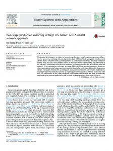
to the output layer (the last layer) through the hidden layer (if any). All of the neural networks used here have a single hidden layer. The nonlinear response of a neuron to its inputs, due to the sigmoidal function, allows for the nonlinear fitting of the function parameterized by the neural network. The error introduced by the use of g instead of f depends on the distance of f to the allowed functions g on B. Given a norm \ · \ on B and given z, the maximum error that we tolerate, we want: FIG. 1. An example of a single-hidden-layer neural network. The spheres symbolize the neurons.

tive codes are the key to a better account of the diurnal cycle. Statistical methods draw interesting prospects to solve this contradiction between speed and accuracy. In this paper we present a fast and accurate method for the computation of longwave flux profiles for clear as well as cloudy situations. The scheme, hereafter referred to as ‘‘NeuroFlux,’’ is based on a neural network technique—the multilayer perceptron (MLP), as defined by Rumelhart et al. (1986). The next section is devoted to a brief description of the MLP. In section 3 we review the radiative transfer equations for longwave fluxes in clear and cloudy atmospheres and describe the features of the neural network–based radiative transfer scheme. In section 4 we present the setup of the datasets on which the parameters of the neural networks are inferred. Section 5 presents the results of flux calculations with NeuroFlux.

∃u ∈ R p , ∀x ∈ A,

\ f (x) 2 g(u, x)\ , z. (2)

The learning phase is devoted to the optimization of the MLP. That is, according to the representativity of the learning set, the algorithm selects a vector u among all of the possible u’s. The so-called back-propagation algorithm enables us to derive the parameters in an iterative way. This method minimizes the quadratic error between the function computed by the network g and the function to be approximated f for a set of patterns for which inputs and ouputs are known—the ‘‘learning set.’’ 3. A neural network model for the longwave radiative transfer a. Longwave radiative transfer equations We restrict ourselves to longwave (LW) radiative transfer modeling. The formal solution of the radiative transfer equation for a stratified cloudless atmosphere in local thermodynamic equilibrium is

E

11

F ↑ (P) 5 p

m dm

[

Neural network techniques, among others, allow us to reduce the number of calculations contained in a function f : A → B, where A , R n and B , R m , by approximating f with a parameterized function g:

E

dn

n

21

2. The multilayer perceptron

3 I ↑n (P0 , m)t n (P0 , P, m) 1

g: A → B

E

P

B n (T P9 )

P0

x → y 5 g(u, x).

(1)

The parameters are gathered in vector u ∈ R and are called ‘‘synaptic weights.’’ These statistical methods have proved their ability to deal with nonlinear problems, in particular the MLP, as defined by Rumelhart et al. (1986). The MLP relies on processors, called ‘‘formal neurons’’ or ‘‘neurons’’ with reference to the biological analogy. A neuron computes a weighted sum of its inputs and transfers this signal through a sigmoidal function (here the hyperbolic tangent). The weights are the parameters in vector u. The neurons are gathered in layers. One or more ‘‘hidden’’ layers of neurons may be introduced between the input layer and the output layer. Figure 1 shows an example of a single-hidden-layer network. Each neuron of layer k receives information from the previous layer k 2 1. Information from the input layer (layer 0) is propagated

and

E E

11

p

F ↓ (P) 5 p

m dm

21

3

0

]t n (P9, P, m) dP9 ]P9

E

]

(3)

dn

n

P

B n (T P9 )

]t n (P9, P, m) dP9, ]P9

(4)

where F ↑ (P) (F ↓ (P)) is the upward (downward) radiative flux at the pressure level P, integrated over the longwave spectrum; I ↑n (P, m) is the monochromatic radiance of frequency n at pressure level P, propagating in a direction such that m is the cosine of the zenith angle; P 0 is the pressure at the surface; n is the frequency; B n (T P ) is the Planck function at temperature T P at pressure level P; and t n (P9, P, m) is the monochromatic flux transmittance for isotropic radiation between the levels of pressure P and P9. By introducing the

NOVEMBER 1998

monochromatic surface emissivity e sn , the surface radiative emission may be expressed by I ↑n (P 0 , m) 5 e snB n (u s ) 1 (1 2 e sn)I ↓n (P 0 , m).

(5)

We divide the atmosphere into N plane-parallel layers from the surface to the TOA. The bottom layer is layer 1 and the top layer is layer N. Following the graybody approximation (Stephens 1978), we describe the cloudiness in a layer k with its horizontal coverage of the grid box n k and its longwave emissivity e k . The only assumptions required are that clouds do not reflect in the longwave and fill the model layer in the vertical. When (n k e k 5 1) in a layer k and (n l e l 5 0) in the other layers, l ± k, the only cloud in the grid box is a black cloud (e k 5 1) in layer k, and it completely covers the grid box (n k 5 1). In this case the vertical upward (downward) fluxes on level i above (below) the black cloud in layer k can be expressed as

E

11

F ↑k (P i ) 5 p

m dm

[

E

dn

n

21

3 B n (T Pk )t n (P k , P, m) 1

E

]t n (P9, P, m) dP9 ]P9

P

B n (T P9 )

Pk

and

E E

11

F ↓k (P i ) 5 p

m dm

E

]

(6)

dn B n (T Pk21 )t n (P k21 , P, m)

P k21

B n (T P9 )

P

]t n (P9, P, m) dP9, ]P9

(7)

where i ranges from 0 (the surface level) to N (the TOA), and P k is the pressure at the top of layer k. The F ↑k ’s (F ↓k ’s) below (upon) the black cloud are the clear-sky fluxes given in (3) and (4). In the general case, in which the effective emissivity n k e k is measured in a layer k by a number between 0 and 1, we use the probability of a clear line of sight between the different levels of calculation. This model of multilayer clouds leads to the following expressions for the upward and downward fluxes: F ↑ (P i ) 5 (1 2 C H,i )F ↑H (P i )

O (1 2 C

H21

1

PC H

k,i

)F ↑k (P i )

k50

l,i

(8)

l5k11

and F ↓ (P i ) 5 (1 2 C i,N )F ↓J11 (P i )

O (1 2 C J11

1

k5i11

TABLE 1. The 20 pressure levels used for radiative computations. Level

Pressure (hPa)

Level

Pressure (hPa)

19 18 17 16 15 14 13 12 11 10

0.0 20.0 40.0 60.8 86.2 119.7 163.6 219.2 286.8 365.4

9 8 7 6 5 4 3 2 1 0

453.1 546.7 642.4 735.3 820.4 892.8 948.5 985.6 1005.2 1013.0

below (above) the level of calculation, C k,i is the probability of a clear line of sight between the levels k and i, and F ↑k (P i ) F ↓k (P i ) is the upward (downward) flux at pressure level P i if the only cloud in the atmosphere was a blackbody in layer k [(6) and (7)]. With this formalism, F ↑0 and F ↓0 correspond to the fluxes in the absence of clouds, described in (3) and (4). The C k,i’s, or cloud fractional coverages, are functions of the ne’s and depend on the way the cloudy layers overlap. Three possibilities are taken into account according to the structure of the clouds: the overlap may be random, maximum, or maximum–random (e.g., Harshvardhan et al. 1987). b. The scheme

n

21

1

1387

CHEVALLIER ET AL.

PC, J

k,i

)F ↓k (P i )

l,i

(9)

l5k21

where H (J) is the index of the highest cloudy layer

Equations (8) and (9) mean that the LW fluxes in the presence of multilayer graybodies, F ↑ and F ↓ , can be deduced from the clear-sky fluxes, F ↑0 and F ↓0 , and from the fluxes in the presence of single-layered black clouds, F ↑k and F ↓k , k . 0. In our approach, the computation of the F ↑k ’s and F ↓k ’s, k $ 0, is based on the MLP, whose basic principles are described in section 2. A first neural network (NN-Clr) computes the clear-sky part of the longwave fluxes, F ↑0 and F ↓0. Then a battery of neural networks (the NN-Cld’s) computes the contribution of every cloudy layer, F ↑k and F ↓k , with k . 0. Each neural network among the NN-Cld’s is dedicated to the calculation of the fluxes, either upward or downward, in the presence of a single black cloud in a specified layer k. The overall fluxes F ↑ and F ↓ are then computed according to (8) and (9). Thus, if M is the number of allowed cloudy layers in the model, our radiative code relies on (1 1 2 3 M) neural networks. In the version we use, the temperature, water vapor, and ozone concentrations are defined in the middle of 19 atmospheric layers (see Table 1) from the TOA to 1013 hPa. The cloudiness is described by the effective emissivity profile [(ne) i ] i51,M . The surface temperature, the mean CO 2 concentration, and the mean longwave surface emissivity are also inputs to the model. The concentrations of the minor gases (e.g., N 2O and CH 4 ) are set to the mean current level. Table 2 describes the neural network architecture. All

1388

JOURNAL OF APPLIED METEOROLOGY

TABLE 2. Architectures of the neural networks in NeuroFlux. Number of neurons (a) Clear-sky neural network Inputs Hidden layer Outputs

60 30 40

(b) Cloudy-sky neural networks Inputs Hidden layer Outputs

Between 1 and 58 20 Between 1 and 19

hidden layers are single. NN-Clr uses the 60 inputs described in the previous paragraph. The 40 outputs include 20 upward fluxes and 20 downward fluxes. The number of inputs and outputs of each one of the (1 1 2M) cloudy networks NN-Cld depends on the position of the considered cloudy layer and on the kind of flux computed. For instance, the computation of the downward flux under a black cloud that top arises at 1005 hPa uses only the temperature at 1013 hPa [see Eq. (7)]. Thus, the input number varies between 1 (computation of the downward flux under a black cloud that top arises at 1005 hPa) and 58 (computation of the upward flux above the previous black cloud). Similarly, the output number varies between 1 and 19. Note that every neural network can compute quantities of the same form:

E

11

Q(P, P b ) 5

m dm

E

dn

n

21

[

3 B n (T Pb )t n (P b , P, m) 1

E

P

Pb

B n (T P9 )

]

]t n (P9, P, m) dP9 , (10) ]P9

where P and P b are the pressures at the boundaries of a given atmospheric layer. One neural network would be sufficient for the computation of all of the F ↑k ’s and the F ↓k ’s, both clear and cloudy, but the specialization of the neural networks in our model in selected fields of the computations improves the accuracy of the neural network simulations because it induces a smaller number of inputs and fewer parameters to set. 4. Training neural networks a. The TIGR (Thermodynamic Initial Guess Retrieval) dataset It appears from the neural network method (described in section 2) that the accuracy of our scheme stems from the statistical characteristics of the training datasets of neural networks NN-Clr and NN-Clds. The essential tool for generating them is the TIGR data bank.

VOLUME 37

The second version of the data bank, TIGR-2 (Achard 1991; Escobar-Munoz 1993), groups together about 1800 atmospheric situations selected from more than 80 000 radiosonde reports collected over 10 years from all parts of the world. The selection method is an iterative process. It relies on a distance D T , which measures the dissimilarity in the temperature profiles of the atmospheric situations. During the first step of TIGR-2’s sampling, the first atmospheric situation in the 80 000 radiosondes is archived. At step n the nth atmospheric situation is selected if its minimum distance D T to the already archived situations is greater than an empirically chosen number Dmin T . Thus, the unequal distribution of the 80 000 radiosondes over space and time disappeared. TIGR-2 can be assimilated into an almost regular networking of the observable atmospheric temperature profiles associated with their corresponding water vapor and ozone profiles. The set is classified into quite homogeneous groups of situations determined from statistical methods, the five airmass classes: tropical (trop), midlatitude (ml1), cold temperate and summer polar (ml2), Northern Hemisphere very cold (pol1), and winter polar (pol2) (Achard 1991). TIGR-2 has been used successfully for retrieving the main thermodynamic parameters from satellite observations with a physicostatistical approach, the Improved Initialization Inversion (3I) (Che´din et al. 1985), and with neural networks [Escobar-Munoz et al. (1993), for the retrieval of temperature profiles, and CabreraMercader and Staelin (1995), for the retrieval of relative humidity]. Nevertheless, two limitations in the design of the TIGR-2 dataset appeared in the framework of the present study. First, the profile selection relies only on a temperature criterion, which does not take care of the variability of the water vapor profiles. Second, the dataset does not contain enough situations with high total water vapor contents. These are mostly below 4 g cm22 , whereas it has been observed that the water vapor content can exceed 7 g cm22 in areas such as the warming pool in the western Pacific. These two limitations are particularly critical in the tropical class. b. A new tropical class TIGR-2’s identified deficiencies mostly impact the tropical class. We undertook to reshape it. The new tropical class has been established according to the following parameters: R the addition of atmospheric situations inferred from satellite data to the initial radiosonde dataset using the 3I algorithm and R a new sampling method that takes the water vapor profiles into account. The TIGR-2 dataset is based upon radiosonde reports, although they do not cover the globe equally. Instruments such as the TIROS-N (Television Infrared Ob-

NOVEMBER 1998

CHEVALLIER ET AL.

1389

FIG. 2. Histograms (40 classes) of the total water vapor contents of the situations in the TIGR-3 tropical class (left) and in the TIGR-2 tropical class (right).

servation Satellite) Operational Vertical Sounder (TOVS) aboard the National Oceanic and Atmospheric Administration (NOAA) polar-orbiting satellites have far better coverage. Traveling through all latitudes and longitudes, TOVS’s are able to observe the properties of the atmosphere over areas poorly described by radiosondes (sparsely populated lands or oceans). The 3I algorithm is designed to retrieve the temperature profile,

layered water vapor contents, surface characteristics, and cloud properties from TOVS-observed radiances. The 3I algorithm has been used for the analysis of a multiyear archive of TOVS satellite data in the framework of the NOAA/National Aeronautical and Space Administration (NASA) Pathfinder program (Scott et al. 1996). The output products for the morning path during July 1987, January 1988, and July 1989 were extracted from our in-house archive. Only the temperature and water vapor information were used from the TOVS 3Iretrieved variables. To design the new tropical class, we first merged two datasets: the 30 000 atmospheric situations of tropical type among the 80 000 radiosonde reports and the tropical-type 3I retrievals extracted from the archive for the three months mentioned above. More than 500 000 tropical situations were collected. We then developed an iterative method to sample the resulting set (Chevallier 1998). The method allowed us to select an atmospheric situation from the 500 000 tropical situations if its temperature profile, its water vapor profile, or the association of the two, was different enough from the already archived profiles. About 900 tropical situations (a relative majority of the 30 000 radiosonde reports) were finally selected due to their high vertical resolution. The histograms of the water vapor contents of the new tropical dataset and of the TIGR-2 tropical class are shown in Figs. 2a and 2b. Note the more regular spread of the points of the 900 situations that have a Gaussian-like shape. We added this tropical set to the four temperate and polar classes of TIGR-2. This new version, ‘‘TIGR-3,’’ contains approximately 2300 situations. c. A better representation of the climatological regimes

FIG. 3. (Top) TIGR-2’s tropical class and (bottom) TIGR-3’s tropical class on a Rossby diagram.

As shown by Stephens et al. (1996), the tropical class of TIGR-2 contains few cases of deep, moist ascent profiles: many of the atmospheric situations contained in the data bank have characteristics of the subsidence process. The irregular representation of the vertical climatological regimes is illustrated in Fig. 3a with a Ross-

1390

JOURNAL OF APPLIED METEOROLOGY

by diagram of TIGR-2’s tropical class. The vertical coordinate Q is the (liquid water) potential temperature, and the horizontal coordinate q is the water vapor mixing ratio. Each TIGR-2 tropical situation is represented by 14 points between 300 and 1013 hPa. The highest part of the profiles appears in the top left corner. For higher pressure levels, the points spread in a triangular shape, indicative of the thermodynamic constraints on the atmospheric profiles. According to their location on the diagram, a point from a situation can be attributed to a particular climatological regime: convection; radiative cooling; upper-tropospheric, meridional transport and subsidence; entrainment; and boundary layer transport (Boers and Prata 1996). Figure 3a shows an irregular spread of the points, indicating an irregular repartition of the TIGR-2 tropical situations on the climatological regimes. Figure 3b presents the same type of projection with the TIGR-3 tropical class. The overall density of the points has increased due to the increased number of atmospheric situations. More importantly, the filling is more regular. We, therefore, have improved the distribution of the different vertical climatological regimes with the new tropical class—in particular, the convection process. d. Surface characteristics, CO 2 concentration, and cloudiness information The learning sets that correspond to the clear and cloudy neural networks, upon which our radiative transfer scheme is based, were selected from TIGR-3. In order to take into account existing discontinuities between the surface temperature and the surface air temperature, we defined a surface temperature for each of the TIGR-3 situations with a random drawing, allowing temperature discontinuities up to 10 K. The mean longwave surface emissivity and the CO 2 concentration were also randomly chosen: between 0.9 and 1.0 and between 200 and 900 ppmv, respectively. For the cloudy-sky learning datasets, black clouds in each atmospheric layer among the 19 were alternately introduced, even though the thermodynamic description of a layer sometimes made the presence of a cloud unlikely. Thus, the learning sets contain atmospheric situations that may never be observed in the atmosphere: they are not only compilations of real atmospheric situations but are also devoted to teach to the networks the computation of longwave radiative fluxes from thermodynamic profiles. For this purpose, it is suitable that a physical phenomenon— such as the presence of a cloud in the atmospheric layers—has in the learning datasets, a regular distribution, rather than a more realistic distribution. e. The vertical pressure grid All atmospheric profiles in the learning datasets have been interpolated from the 40 pressure-level grid on which they are archived in the TIGR dataset, on the grid

VOLUME 37

that NeuroFlux uses. We defined NeuroFlux in such a way that each version of the scheme is dedicated to a specified vertical pressure grid. This is not the case with the usual wideband models, which allow the pressure grid to be changed easily. In the versions of NeuroFlux that we use in this paper, the temperature, water vapor, and ozone profiles are discretized in the middle of 19 layers, as shown in Table 1. The pressure levels of this grid are fixed. Surface pressures less than 1013 hPa can be introduced with a blackbody at the ground pressure: the altitude is treated in the same way as is cloudiness. If one wants to choose a different vertical grid, one has to retrain the networks on this new grid. The most time-consuming computations are absorbed in the learning phase: once it is done, the method is very fast. The sigma-pressure-level grids used in most GCMs can be introduced easily by adding the surface pressure to the inputs of the scheme. f. Computation of the radiative characteristics of the learning datasets We used two radiative forward models to obtain the radiative characteristics of these profiles [the LW fluxes from (3), (4), (6), and (7)]: the ECMWF wideband operational scheme (Morcrette 1991; Zhong and Haigh 1995) and the Automatized Atmospheric Absorption Atlas line-by-line model (4A) (Scott and Che´din 1981; Tournier et al. 1995). In the following, the ECMWF wideband model will be referred to as ‘‘the WBM.’’ It uses averages of the absorption parameters over spectral intervals of hundreds of inverse centimeters, whereas 4A takes into account each absorption line of the different atmospheric constituents. In an earlier paper, we also presented some results of the neural network model using a narrowband model (Che´ruy et al. 1996a). The WBM refers to nine spectral intervals, for which absorption by H 2O, O 3 , CO 2 , CH 4 , N 2O, CFC-11, and CFC-12 is accounted. This model was calibrated against the Geophysical Fluid Dynamics Laboratory (Schwarzkopf and Fels 1991) line-by-line results. The parameterization of the water vapor has been improved recently by Zhong and Haigh (1995). This code is fast enough to be used in operational weather forecasts (at ECMWF) and for climate simulations (in the LMD general circulation model). The 4A model takes into account all radiatively active atmospheric constituents, the H 2O, N 2 , and O 2 continua and the CO 2 line coupling. This line-by-line and layerby-layer method allows us to quickly restore monochromatic optical depths for each absorbing gas in each atmospheric layer for realistic atmospheric situations: the most time-consuming computations have been absorbed, once and for all, by precomputations, the results of which constitute the 4A atlas. The complete validation of the method for high spectral resolution is based on comparisons with the high-resolution interferometer sounder (Smith et al. 1988) measurements. The 4A mod-

NOVEMBER 1998

CHEVALLIER ET AL.

1391

FIG. 4. Comparison between the computations of 4A and WBM on 1032 radiosonde reports (cooling rates from the WBM minus cooling rates from 4A, in K day21 ). Results are shown by airmass class: (a) tropical, (b) midlatitude, and (c) polar.

el is much more accurate than the WBM, but its lengthy computing time forbids its use for long-term global calculations. In numerical models of atmospheric circulation, the radiative cooling rates are used instead of the fluxes themselves. The cooling rates, in K day21 , are the divergences of the radiative fluxes. They equal the rate at which energy is lost by the atmosphere from radiation: C(P) 5 2

g ]F(P) , C p ]P

(11)

where F(P) 5 F ↑ (P) 2 F ↓ (P) is the net flux, C p is the heat capacity at constant pressure, and g is the gravitational acceleration. To compare the two codes, we have computed the mean and standard deviation of their computations of the fluxes and cooling rates for 1032 radiosonde reports (Moulinier 1983). These observations—in the following set ‘‘S’’—cover a wide range of atmospheric situations.

As we did for the 80 000 radiosonde reports, we classified S into the five TIGR airmass classes. For the forthcoming statistics, the two midlatitude classes (ml1 and ml2) are mixed in a single midlatitude class and the two polar classes (pl1 and pl2) are mixed in a single polar class. Thus, the 1032 radiosonde reports are divided into three airmass classes: tropical (265 situations), midlatitude (509 situations), and polar (258 situations). The radiative computations of these atmospheric situations are performed cloudless. The atmosphere is divided into the 19 layers from Table 1. For 4A, the monochromatic optical depths are first computed on 39 layers from the archived optical depths before being interpolated into the 19 layers. Figure 4 shows the differences between the two codes, 4A and WBM, for the computation of cooling rates, and Table 3 for the outgoing longwave radiances (OLRs) and downward longwave radiance at the surface (DLR). The absolute value of the sytematic differences

1392

JOURNAL OF APPLIED METEOROLOGY

VOLUME 37

TABLE 3. Mean (m) and standard deviation ( s) of 4A (line by line) and the WBM (band model) for the computation of the (a) OLR and (b) DLR for 1032 atmospheric situations. Fluxes in watts per square meter. Tropical

Midlatitude

Polar

Model

m

s

m

s

m

s

(a) WBM 4A WBM-4A

265.5 263.3 2.1

16.4 16.4 0.7

227.7 226.1 1.6

18.9 18.8 0.7

188.4 187.7 0.7

14.5 14.6 1.1

(b) WBM 4A WBM-4A

314.9 312.5 2.4

48.6 47.4 2.0

221.7 222.9 21.3

34.7 33.0 1.9

155.5 158.7 23.3

19.9 19.7 0.8

between the cooling rates from 4A and from WBM reaches 0.4 K day21 at 300 hPa and near the ground in the tropical class (Fig. 4). The sign changes around 500 hPa. Compared with 4A, the WBM tends to cool the high troposphere and heat the boundary layer. The standard deviations are of the order of 0.2 K day21 above 600 hPa and increase below. Overall, the differences increase with the water vapor content. For the OLR, the mean difference is between 2.1 W m22 in the tropical class and 0.7 W m22 in the polar class. The standard deviations are about 0.7 W m22 . For the DLR, the differences are larger, with an rms of the order of 3 W m22 .

For the computation of OLR and DLR (Table 4), the standard deviations are similar to those between WBM and 4A: 1.0 W m22 for OLR and 1.6 W m22 for DLR. The biases, whose absolute value is less than 1.0 W m22 , are significantly smaller. We checked the accuracy of the cloudy neural networks by artificially adding black clouds in the radiosondes and comparing the corresponding computations of the WBM and NeuroFlux-A. The neural network– based model exhibits, with WBM, differences similar to the ones observed in clear-sky situations (results not shown).

5. Performances

b. NeuroFlux-A: Comparisons with the WBM using TOVS 3I global data

a. NeuroFlux-A: Comparisons with WBM using radiosonde data The F ↑n’s and the F ↓n’s for the training of the neural networks were first computed with WBM. These learning datasets led to a first version of our neural network model, called NeuroFlux-A. Radiative fluxes obtained by using either NeuroFluxA or WBM have been compared for the 1032 radiosonde reports from the set S. None of them was used in the learning datasets of the neural networks. For the three airmass classes, we computed the biases and standard deviations of the differences between the radiative calculations of NeuroFlux-A and WBM. The computations are performed cloudless. Results are shown in Fig. 5. The standard deviations are about 0.2 K day21 . The absolute value of the biases are less than 0.05 K day21 in the midlatitude and polar classes. In the tropical class the absolute value is slightly higher but less than 0.1 K day21 except near the ground, where the bias reaches 20.2 K day21 . Compared with Fig. 4, the standard deviations are similar, but the biases are significantly smaller. Because NeuroFlux is based on principles that differ greatly with the principles of WBM, the maximum errors are also interesting characteristics of the validation. For NeuroFlux-A, the maximum error in the troposphere equals 1.8 K day21 , less than the maximum error of the WBM compared with 4A, which reaches 2.9 K day21 .

To study the robustness of the method, we have extended the previous comparisons between the two models, WBM and NeuroFlux-A, to an observation dataset consisting of two years of global data. To do so, we used the geophysical parameters inferred from TOVS data, actually the TOVS 3I–retrieved products morning path, obtained from April 1987 to March 1989 (Scott et al. 1996). The computation of the radiative fluxes from the TOVS 3I products using WBM is explained in Che´ruy et al. (1996b). Each month groups together hundreds of thousands of tropical, midlatitude, and polar clear and cloudy atmospheric situations. We computed the global monthly mean error of the instantaneous differences. For upward flux calculations (Fig. 6a), the rms of differences between NeuroFlux-A and WBM remains between 1 and 2 W m22 , which represents less than 0.6% of the upward flux values. For downward fluxes (Fig. 6b), the results are similar with a larger difference around 500 hPa of about 4%. This larger error is due to both a particularity in the TOVS 3I–retrieved profiles and the way NeuroFlux parameters are inferred. The water vapor profiles inferred from TOVS 3I—actually amounts in four coarse layers—sometimes present important discontinuities at 500 hPa. Now, in their computations, the neural networks exploit the correlations that usually exist in the learning datasets between successive water vapor specific humidities in the water va-

NOVEMBER 1998

1393

CHEVALLIER ET AL.

FIG. 5. Comparison between the computations of NeuroFlux-A and WBM on 1032 radiosonde reports (cooling rates from NeuroFlux-A minus cooling rates from the WBM, in K day21 ). Results are shown by airmass class: (a) tropical, (b) midlatitude, and (c) polar.

por profiles. A coarse resolution of the profile degrades both the correlations and the quality of the results. The difference between outputs of NeuroFlux-A and WBM decreases below 1% near the ground. For the calculation of cooling rates, deviations are less than 0.3

K day21 . We obtained similar results with the evening path data. The neural network method performs equally for the whole period. Note that the error does not particularly decrease either during July 1987 or during January

TABLE 4. Mean (m) and standard deviation ( s) of NeuroFlux-A and the WBM for the computation of the (a) OLR and (b) DLR for 1032 atmospheric situations. Fluxes in watts per square meter. Tropical

Midlatitude

Polar

Model

m

s

m

s

m

s

(a) NeuroFlux-A NeuroFlux-A–WBM

265.9 0.5

16.3 1.2

228.6 0.8

18.9 0.8

189.1 0.8

14.3 0.9

(b) NeuroFlux-A NeuroFlux-A–WBM

314.6 20.4

49.0 1.6

221.8 0.1

34.2 1.6

155.9 0.5

19.7 2.0

1394

JOURNAL OF APPLIED METEOROLOGY

VOLUME 37

between WBM and 4A, the standard deviations are similar, but the biases are significantly smaller. The validation of the NeuroFlux-B cloudy-skies neural networks gave similar results (not shown). Therefore, the neural network parameterization using line-by-line computations appears to be more accurate than the classic parameterization of WBM. d. NeuroFlux-B: Doubling CO 2 concentrations experiment

1988, although these two months were used for the extension of TIGR-2. The stability of the method enables us to use the code for long-term and global simulations, as is done in numerical models of atmospheric circulation.

The computing time of NeuroFlux-B reference code (4A) forbids global long-term validations of NeuroFluxB as was done with NeuroFlux-A, though other kinds of validations are possible: in particular, the classic sensitivity study doubling concentrations of CO 2 . Indeed, for a climate model it is particularly important to obtain the correct tendency to changes in CO 2 concentrations. To assess this sensitivity, both 4A and NeuroFlux-B were used to compute the differences in cooling rates for set S resulting from doubling concentrations of CO 2 from its current level of 355 to 710 ppmv. For brevity, only the results for the tropical class are shown. Figure 8a presents the mean and standard deviation of the 4A computations. They show known features of the atmospheric response to increased CO 2 (e.g., Schlesinger and Mitchell 1987): the stratosphere cools and the troposphere warms. Figure 8b presents NeuroFlux-B computations and the corresponding error. NeuroFlux-B reproduces the stratospheric tendency well with negligible biases and standard deviations. In the troposphere, where the change in cooling rate is far smaller, the error is characterized by a standard deviation of about 0.03 K day21 , that is, more than half of the rms signal (about 0.05 K day21 ). Nevertheless, the error bias is less than 0.01 K day21 when the mean signal is about 0.04 K day21 . Every paramerization method brings noise into the realizations of a function f to be computed. The results of NeuroFlux-B validation show that the noise introduced by the neural networks is small for computations of individual fluxes or cooling rates but is not negligible in sensitivity tests, though the mean tendency is well reproduced by the method. This is very fundamental for climate studies.

c. NeuroFlux-B: Comparisons with 4A

e. Computing time

For NeuroFlux-B, the longwave fluxes of the learning datasets for the neural networks are computed with 4A. We carried out the validation of the parameterization on the 1032 radiosonde reports from the set S. Figure 7 shows the results for the computation of the cooling rates, and Table 5 shows the results for the computation of the OLR and DLR in clear situations. Although the training model is much more accurate, the differences between NeuroFlux-B and 4A are similar to the ones between NeuroFlux-A and WBM. Compared to the ones

The architecture of the neural networks enables fast computations with modern computers in spite of the number of parameters the neural networks include. We compared the computing times of NeuroFlux-A and NeuroFlux-B to the computing times of WBM and 4A, respectively. The computing times of our schemes vary according to the number of cloud layers since for each additional layer in the atmosphere the algorithm includes two more neural networks to perform the computations. Figure 9

FIG. 6. Evolution of the rms of the differences between NeuroFluxA and WBM for the computation of (a) upward fluxes and (b) downward fluxes during two years of global data (W m22 ). Values are given on a 20 pressure-level grid.

NOVEMBER 1998

1395

CHEVALLIER ET AL.

FIG. 7. Comparison between the computations of NeuroFlux-B and 4A on 1032 radiosonde reports (cooling rates from NeuroFlux-B minus cooling rates from 4A, in K day21 ). Results are shown by airmass class: (a) tropical, (b) midlatitude, and (c) polar.

shows the gain in rapidity of NeuroFlux-A compared with the WBM versus the number of cloudy layers. The computations were performed on a CRAY C98. For clear skies, the neural network method saves computing time by a factor of 32, as compared with the initial scheme. For 15 cloudy layers, the computing time is smaller by a factor of 16. For an entire month of TOVS

data, with both clear and cloudy situations, NeuroFluxA is 22 times as fast. Since the architectures of NeuroFlux-B and NeuroFlux-A neural networks are the same, their computing times are exactly the same, although the code NeuroFlux-B simulates—the 4A line-by-line model— is much more accurate. The neural networks allow us

TABLE 5. Mean (m) and standard deviation ( s) of NeuroFlux-B and 4A for the computation of the (a) OLR and (b) DLR for 1032 atmospheric situations. Fluxes in watts per square meter. Tropical

Midlatitude

Polar

Model

m

s

m

s

m

s

(a) NeuroFlux-B NeuroFlux-B–4A

263.6 0.3

16.4 1.0

226.4 0.3

18.9 0.9

188.0 0.4

14.2 1.1

(b) NeuroFlux-B NeuroFlux-B–4A

312.8 0.3

47.3 1.0

223.1 0.1

33.1 1.2

158.5 20.2

19.2 1.6

1396

JOURNAL OF APPLIED METEOROLOGY

VOLUME 37

FIG. 9. Speed ratio between WBM and NeuroFlux-A (computing time of the WBM on computing time of NeuroFlux-A). Computation performed on a Cray C98 for 200 atmospheric situations.

FIG. 8. Effect on the cooling rates due to doubled concentrations of carbon dioxide from current level (355 ppmv) for the 509 midlatitude situations of set S. (a) Computation with 4A, mean, plus or minus one standard deviation (cooling rates at 355 ppmv minus cooling rates at 710 ppmv). (b) Corresponding NeuroFlux-B error (difference in cooling rates from NeuroFlux-B minus difference in cooling rates from 4A). Cooling rates in K day21 .

to benefit from the accuracy of the line-by-line model while drastically reducing the required computing time. Compared with 4A, the required computing time is divided by a factor of 10 6 .

putations were used for both training and controlling the quality of two neural network models—NeuroFluxA and NeuroFlux-B. Global-scale comparisons with the wideband model showed that the error associated with our parameterization stays significantly below the error commonly admitted for a wideband model. By comparison, the discrepancies observed between various wideband models in the 1991 ICRCCM-2 exercise (Ellingson and Ellis 1991) were significantly larger. For example, the discrepancies reach 12% for the downward flux at the tropopause of a midlatitude summer profile, whereas we estimated the error introduced by our parameterization to be less than 5% in similar conditions. Compared with WBM, the use of neural networks trained with the lineby-line scheme leads to a more accurate parameterization of longwave radiative processes: the systematic differences between the parameterized radiative transfer scheme and the line-by-line model are significantly reduced, while the standard deviations are similar. The impact of these differences is currently evaluated in the framework of the LMD GCM. The decrease of the biases should induce a reduction of the systematic undesirable tendencies of the simulations, such as excessive cooling in the high troposphere, as shown in Fig. 4. The major advantage of NeuroFlux is its reduction in computing time; it is 22 times faster than WBM and 10 6 times faster than 4A. NeuroFlux enables more frequent calls to the longwave routines and, thus, takes the diurnal cycle into account better.

6. Conclusions We showed that neural networks can be used successfully to derive the vertical atmospheric longwave radiative budget from the TOA to the surface. We used a wideband model and a line-by-line model for the longwave radiative transfer—two codes differing widely in their computing time requirements and accuracy—to compute profiles of longwave fluxes and cooling rates from the TOA to the surface. The results of these com-

Acknowledgments. The authors wish to thank J.-J. Morcrette for making the different versions of the ECMWF radiative code available to them and for fruitful discussions. The most time-consuming computations were performed on IDRIS/CNRS (Institut du De´veloppement et des Ressources en Informatique Scientifique Centre National de la Recherche Scientifique) computers.

NOVEMBER 1998

CHEVALLIER ET AL. REFERENCES

Achard, V., 1991: Trois proble`mes cle´s de l’analyse 3D de la structure thermodynamique de l’atmosphe`re par satellite: Mesure du contenu en ozone; classification des masses d’air; mode´ lisation hyper rapide du transfert radiatif. Ph.D. thesis, Universite´ Paris VI, 168 pp. [Available from LMD, Ecole Polytechnique, 91128 Palaiseau Cedex, France.] Boers, R., and J. Prata, 1996: Thermodynamic structure of the maritime troposphere around the Australian continent. Int. J. Climate, 16, 1–18. Cabrera-Mercader, C. R., and D. H. Staelin, 1995: Passive microwave relative humidity retrievals using feedforward neural networks. IEEE Trans. Sci. Remote Sens., 33, 1324–1326. Cess, R. D., and Coauthors, 1993: Uncertainties in carbon dioxide radiative forcing in atmospheric general circulation models. Science, 262, 1252–1255. Che´din, A., N. A. Scott, C. Wahiche, and P. Moulinier, 1985: The Improved Initialization Inversion method: A high-resolution physical method for temperature retrievals from satellites of the TIROS-N series. J. Climate Appl. Meteor., 24, 128–143. Che´ruy, F., F. Chevallier, J.-J. Morcrette, N. A. Scott, and A. Che´ din, 1996a: A fast method using neural networks for computing the vertical distribution of the thermal component of the Earth radiative budget (in French). C. R. Acad. Sci. Paris, 322 (IIb), 665–672. , , N. A. Scott, and A. Che´din, 1996b: Use of the vertical sounding in the infrared for the retrieval and the analysis of the longwave radiative budget. IRS ’96: Current Problems in Atmospheric Radiation, W. L. Smith and K. Stamnes, Eds., A. Deepak, 375–376. Chevallier, F., 1998: La mode´lisation du transfert radiatif a` des fins climatiques: Une nouvelle approche fonde´e sur les re´seaux de neurones artificiels. Ph.D. thesis, University Paris VII, 225 pp. [Available from LMD, Ecole Polytechnique, 91128 Palaiseau Cedex, France.] Ellingson, R. G., and J. Ellis, 1991: The intercomparison of radiation codes used in climate models: Longwave results. J. Geophys. Res., 96 (D5), 8929–8953. Escobar-Munoz, J., 1993: Base de donne´es pour la restitution de variables atmosphe´ riques a` l’e´chelle globale. E´ tude sur l’inversion par re´seaux de neurones des donne´es des sondeurs verticaux atmosphe´riques satellitaires pre´sents et a` venir. Ph.D thesis, Universite´ Paris VII, 190 pp. [Available from LMD, Ecole Polytechnique, 91128 Palaiseau Cedex, France.] , A. Che´din, F. Che´ruy, and N. A. Scott, 1993: Re´seaux de neurones multi-couches pour la restitution de variables thermodynamiques atmosphe´riques a` l’aide de sondeurs verticaux satellitaires. C. R. Acad. Sci. Paris, 317 (IIb), 911–918. Harshvardhan, D. A. Randall, and T. G. Corsetti, 1987: A fast radiation parameterization for atmospheric circulation models. J. Geophys. Res., 92, 1009–1016. Morcrette, J.-J., 1991: Radiation and cloud radiative properties in the

1397

European Centre for Medium-Range Weather Forecasts forecasting system. J. Geophys. Res., 96 (D5), 9121–9132. Moulinier, P., 1983: Analyse statistique d’un vaste e´ chantillonnage de situations atmosphe´riques sur l’ensemble du globe. LMD Internal Note 123, 30 pp. [Available from LMD, Ecole Polytechnique, 91128 Palaiseau Cedex, France.] Rumelhart, D. E., G. E. Hinton, and R. J. Williams, 1986: Learning internal representations by error propagation. Parallel Distributed Processing: Explorations in the Macrostructure of Cognition 1, D. E. Rumelhart and McClelland, Eds., MIT Press, 318–362. Sadourny, R., and K. Laval, 1984: January and July performances of the LMD general circulation model. New Perspectives in Climate Modelling, A. L. Berger and C. Nicolis, Eds., Elsevier, 173–198. Schlesinger, M. E., and J. F. B. Mitchell, 1987: Climate model simulations of the equilibrium climatic response to increased carbon dioxide. Rev. Geophys., 25, 760–798. Schwarzkopf, M. D., and S. B. Fels, 1991: The simplified exchange method revisited: An accurate, rapid method for computation of infrared cooling rates and fluxes. J. Geophys. Res., 96 (D5), 9075–9096. Scott, N. A., and A. Che´din, 1981: A fast line-by-line method for atmospheric absorption computations: The Automatized Atmospheric Absorption Atlas. J. Appl. Meteor., 20, 802–812. , and Coauthors, 1996: Re-analysis of a multi-year archive of TOVS/ NOAA satellite data for climate studies. Proc. Global Energy and Water Cycle Symp., Washington, DC, World Meteorological Organization, 375–376. Smith, W. L., H. M. Woolf, H. B. Howell, H. L. Huang, and H. E. Revercomb, 1988: The simultaneous retrieval of atmospheric temperature and water vapor profiles—Applications to measurements with the high spectral resolution infrared sounder (HIS). RSRM ’87: Advances in Remote Sensing Retrieval Methods, A. Deepak, H. Fleming, and J. S. Theon, Eds., A. Deepak, 189–202. Stephens, G. L., 1978: Radiation profiles in extended water clouds. II: Parameterization schemes. J. Atmos. Sci., 35, 2123–2132. , D. L. Jackson, and I. Wittmeyer, 1996: Global observations of upper-tropospheric water vapor derived from TOVS radiance data. J. Climate, 9, 305–325. Tournier, B., R. Armante, and N. A. Scott, 1995: Stransac-93, 4A93. De´veloppement et validation des nouvelles versions des codes de transfert radiatif pour application au projet IASI. LMD Internal Note 201, 43 pp., [Available from LMD, Ecole Polytechnique, 91128 Palaiseau Cedex, France.] Wilson, C. A., and J. F. B. Mitchell, 1986: Diurnal variation and cloud in General Circulation Model. Quart. J. Roy. Meteor. Soc., 112, 347–369. Zhong, W., and J. D. Haigh, 1995: Improved broadband emissivity parameterization for water vapor cooling rate calculations. J. Atmos. Sci., 52, 124–138.