Neural Networks 21 (2008) 535–543 www.elsevier.com/locate/neunet
2008 Special Issue
Neural network approach for robust and fast calculation of physical processes in numerical environmental models: Compound parameterization with a quality control of larger errorsI,II Vladimir M. Krasnopolsky a,b,∗ , Michael S. Fox-Rabinovitz b , Hendrik L. Tolman c , Alexei A. Belochitski b a Science Applications International Corporation at Environmental Modeling Center, National Centers for Environmental Prediction, National Oceanic and
Atmospheric Administration, MD, USA b Earth System Science Interdisciplinary Center, University of Maryland, MD, USA c Environmental Modeling Center, National Centers for Environmental Prediction, National Oceanic and Atmospheric Administration, MD, USA
Received 2 August 2007; received in revised form 13 November 2007; accepted 13 December 2007
Abstract Development of neural network (NN) emulations for fast calculations of physical processes in numerical climate and weather prediction models depends significantly on our ability to generate a representative training set. Owing to the high dimensionality of the NN input vector which is of the order of several hundreds or more, it is rather difficult to cover the entire domain, especially its “far corners” associated with rare events, even when we use model simulated data for the NN training. Moreover the domain may evolve (e.g., due to climate change). In this situation the emulating NN may be forced to extrapolate beyond its generalization ability and may lead to larger errors in NN outputs. A new technique, a compound parameterization, has been developed to address this problem and to make the NN emulation approach more suitable for long-term climate prediction and climate change projections and other numerical modeling applications. Two different designs of the compound parameterization are presented and discussed. c 2008 Elsevier Ltd. All rights reserved.
Keywords: Neural networks; Numerical modeling; Climate; Weather; Waves; Data assimilation
1. Introduction This paper describes an interdisciplinary study. This study follows upon our previous works presented in the previous papers of the authors (e.g., Krasnopolsky, Chalikov, and Tolman (2002) and Krasnopolsky, Fox-Rabinovitz, and Chalikov (2005)). In these works we developed a new approach, introducing nonlinear statistical learning techniques (NNs) into tremendously complex and time consuming numerical models, describing one of the most complex, multidimensional, I MMAB Contribution No. 258. II An abbreviated version of some portions of this article appeared in
Krasnopolsky, Fox-Rabinovitz, and Belochitski (2007) as part of the IJCNN 2007 Conference Proceedings, published under IEE copyright. ∗ Tel.: +1 301 763 8000; fax: +1 301 763 8545. E-mail address:
[email protected] (V.M. Krasnopolsky). c 2008 Elsevier Ltd. All rights reserved. 0893-6080/$ - see front matter doi:10.1016/j.neunet.2007.12.019
and essentially nonlinear systems (climate/weather system) known to the modern science. This new approach introduces fast and accurate NN emulations of time consuming original model components into numerical climate/weather models. As a result, the model computational performance improves significantly without a detriment to the quality of model predictions. This applied research (and the current study) has a clearly formulated practical goal: to improve computational performance of operational weather prediction and climate simulation models by using accurate, fast, and robust NN emulations substituting the time consuming original components of the models. 1.1. Climate models and model physics One of the main problems of development and implementation of high-quality high-resolution environmental models is the complexity of physical (chemical and biological) processes
536
V.M. Krasnopolsky et al. / Neural Networks 21 (2008) 535–543
involved. For example, for the state-of-the-art climate model, the National Center for Atmospheric Research (NCAR) Community Atmospheric Model (CAM) (see the special issue on the National Center for Atmospheric Research Community Climate Model in the Journal of Climate, 11 (6) 1998, for the description of the model), calculation of a model physics package takes about 70% of the total model computations. For this and other numerical models neural network (NN) techniques have been developed (Krasnopolsky et al., 2002, 2005; Tolman, Krasnopolsky, & Chalikov, 2005; Krasnopolsky & FoxRabinovitz, 2006; Krasnopolsky, 2007) for speeding up the calculations of model physics (i.e., deterministic or first principle components of atmospheric and oceanic numerical models describing physical processes) up to two to five orders of magnitude. The speed-up is achieved through the development of NN emulations of model physics. Tremendous complexity, multidimensionality, and nonlinearity of the climate/weather system and numerical models describing this system lead to complexity and multidimensionality of our NN emulations and data sets that are used for their development and validation. Also, the validation procedure for developed NN emulations becomes more complicated because, after their development, they are supposed to work in a complex and essentially nonlinear numerical model. The development of NN emulations of model physics depends significantly on our ability to generate a representative training set to avoid using NNs for extrapolation beyond the domain covered by the training set. Owing to the high dimensionality of the input domain (i.e., dimensionality of the NN input vector) which is of the order of several hundreds or more, it is difficult if not impossible to cover the entire domain, especially its “far corners” associated with rare or extreme events, even when we use model simulated data for the NN training. Also, the domain may change with time as in the case of climate change. In such situations the emulating NN may be forced to extrapolate beyond its generalization ability which may lead to larger errors in NN outputs and, as a result, to errors in the numerical models in which they are used. 1.2. NN emulations of model physics We have developed NN emulations of major components of climate model physics (Krasnopolsky et al., 2005; Krasnopolsky & Fox-Rabinovitz, 2006; Krasnopolsky, 2007) for the widely recognized and used NCAR CAM. Specifically, we developed the NN emulations of the NCAR CAM long wave radiation (LWR) and short wave radiation (SWR) parameterizations which are the most time consuming components of model physics describing the propagation of electromagnetic radiation in the Earth’s atmosphere. Both original (i.e. used in the current version of NCAR CAM) LWR and SWR parameterizations are physically based process models. They may be considered mathematically as a continuous or almost continuous mapping between two vectors X (input vector) and Y (output vector) and symbolically can be written as: Y = M(X );
X ∈ Rn , Y ∈ Rm
(1)
where M denotes the mapping, n is the dimensionality of the input space (the number of NN inputs), and m is the dimensionality of the output space (the number of NN outputs). The simplest multi-layer perceptron (MLP) NN with one hidden layer and linear neurons in the output layer can be used as a generic analytical nonlinear approximation or model for the mapping (1) (Funahashi, 1989; Hornik, 1991). In our application, the possibility to use the simplest MLP NN is very important because the complexity and high dimensionality of the problem impose significant limitations on the arsenal of NN techniques and statistical metrics that can be used in our study. Also, the choice of statistical metrics used is determined and conditioned by those used for estimating errors and performances in the climate/weather modeling; this is a consequence of the interdisciplinary nature of the study. The developed NN emulations for LWR and SWR are highly accurate and much more computationally efficient than the original NCAR CAM LWR and SWR, respectively. For example, the NN emulations using 50 neurons (NN50) for the LWR NN emulation and 55 neurons (NN55) for the SWR NN emulation in the single hidden layer provide, if run separately (code by code comparison) at every model physics time step (1 hour), the speed-up of ∼150 times for LWR and of ∼20 times for SWR as compared with the original LWR and SWR, respectively. These NNs have each more than 200 inputs and about 50 outputs (as many as the original LWR and SWR parameterizations which they emulate and substitute). The number of NN weights (or dimensionality of the NN training space) for these NNs reaches 10,000–20,000. The dimensionality is higher for NNs with a larger hidden layer and/or for models with higher vertical resolution (Krasnopolsky et al., 2005; Krasnopolsky, 2007). All details of creating the training, validation, and test sets and of selecting the NN architecture are discussed in Krasnopolsky (2007). Here we only mention that each of these independent data sets consist of more than 100,000 records. Each record is a combination of an input vector X with more than 200 components and an output vector Y with about 50 components. Problems associated with normalizing multiple outputs of different nature and with choosing an error metric and a training algorithm, when dealing with such highdimensional mappings and long training sets, are discussed in details in our earlier paper (Krasnopolsky & Fox-Rabinovitz, 2006). The results of long multi-decadal climate simulations performed with NN emulations for both LWR and SWR, i.e., for the full model radiation, have been validated against the parallel control NCAR CAM simulation using the original LWR and SWR. Almost identical results have been obtained for these parallel 50-year climate simulations (Krasnopolsky, FoxRabinovitz, & Belochitski, 2007). In another numerical model, an ocean wind wave model which is used for the simulation and forecast of ocean waves, the nonlinear wave–wave interaction represents a significant computational “bottleneck”. An accurate calculation of this component requires roughly 103 –104 times more computational effort than all other aspects of the wave model combined.
V.M. Krasnopolsky et al. / Neural Networks 21 (2008) 535–543
For over 40 years researchers have been trying to get economical approximations for the nonlinear four-wave interactions. The only feasible result so far has been the direct interaction approximation (DIA) parameterization, which dates back more than 20 years. This simple parameterization with computational efforts comparable to all other aspects of a wave model combined makes wave modeling economically feasible, but also limits the potential of further model development. All other mapping approaches that were developed before have failed in the sense that none of these methods resulted in a stable model integration. It is therefore a significant achievement that the method presented here does provide stable model integration. As the (exact or approximate) nonlinear wave–wave interaction can be considered as a continuous mapping (1), we applied a NN technique and developed a NN emulation of the exact nonlinear interactions. The NN emulation is about five orders of magnitude faster than the exact interactions, and hence comparable in costs to the simple DIA parameterization (Krasnopolsky et al., 2002; Tolman et al., 2005). Unlike the simple DIA parameterization, the NN approximation retains major details of the exact interactions. This NN emulation was further validated through integration for a limited period in the National Centers for Environment Prediction (NCEP) operational wave model (WAVEWATCH III). 1.3. Accuracy and quality control of NN emulations The accuracy of NN emulations of model physics depends significantly on our ability to generate a representative training set to avoid using NNs for extrapolation beyond the domain covered by the training set. Owing to the high dimensionality of the input domain (i.e., dimensionality of the NN input vector X ) which is of the order of several hundreds or more, it is difficult if not impossible to cover the entire domain, which may have a very complex shape, even when we use model simulated data for the NN training. Also, the domain may change with the evolution of the system during a simulation period. In such situations the emulating NN may be forced to extrapolate beyond its generalization ability which may lead to larger errors in NN outputs and correspondingly in the numerical model simulations in which NN emulations are used. The developed NN emulations are very accurate. Larger errors and outliers (a few extreme errors) in NN emulation outputs occur only when NN emulations are exposed to inputs not represented sufficiently in the training set. These errors have a very low probability (see Fig. 3) and are distributed randomly in space and time. However, when long multi-decadal climate simulations are performed and NN emulations are used in a very complex and essentially nonlinear climate model for such a long integration time, the probability for occurrence of larger errors and the probability of their undesirable impact on the model simulations increase. As we learned from our experiments with NCAR CAM, the model was in many but not in all cases (shown, for example, in Fig. 7 of Section 2) robust enough to overcome such randomly distributed errors without their accumulation in time. However, for these few cases, it is still essential to develop and use for NN emulations an internal
537
quality control (QC) procedure capable of controlling their larger errors. In another application of a NN approximation to nonlinear interactions in a wave model, the model did not prove sufficiently robust to retain stability for time integrations of even a few hours. Thus, in this model, introducing an internal QC method for identifying and controlling larger NN emulation errors is especially essential for the successful application of NN emulation of the model physics (Tolman & Krasnopolsky, 2004). Therefore, it is essential to introduce a QC procedure, which can predict and eliminate larger errors of NN emulations during the integration of highly nonlinear numerical models, not just relying upon the robustness of the model that can vary significantly for different models. Such a mechanism would make our NN emulation approach more reliable, robust, and generic. In this paper, we introduce a compound parameterization (CP) which combines NN emulation with a QC technique. We present two different designs of CP both based on the use of NN techniques. We also discuss the possibility of using CP as a tool for introducing a dynamical adjustment of NN emulations to climate change. In Section 2 we introduce the CP approach and discuss its application and versions as well as its validation on an independent data set and through NCAR CAM and WAVEWATHC III simulations. Conclusions and discussion are presented in Section 3. 2. The compound parameterization approach for reducing the amount of larger errors in NN emulations 2.1. Two-step validation procedure for NN emulations and CP The final goal of our developments is a stable functioning of the NN emulation in the complex nonlinear numerical model for a sufficiently long time and the similarity of the model results produced with the original component (the control run) and with the NN emulation of this component. For such a situation, the high accuracy of a NN emulation obtained on an independent test set does not guarantee its stable performance in a numerical model. Thus, in our case, a reasonably good accuracy of NN emulation on a test set is a necessary but not sufficient condition for the satisfactory validation of NN emulation. This is only the first step of the two-step validation procedure used for the validation of the developed NN emulations in our previous studies (e.g. Krasnopolsky et al. (2005) and Krasnopolsky and Fox-Rabinovitz (2006)), and also used for validation of CPs developed in this study. The second and the most important step of the validation procedure is the validation of the model run with NN emulation vs. the control run with the original parameterization. During this second validation step, the run with the NN emulation (or with CP) should demonstrate, in addition to its stable performance, a close similarity of all simulated results to those of the control run. 2.2. CP designs and their validation on independent data sets CP consists of the following three components: the original parameterization, its NN emulation, and a quality control (QC) block (see Figs. 1 and 4). During a routine numerical model
538
V.M. Krasnopolsky et al. / Neural Networks 21 (2008) 535–543
Fig. 1. Compound parameterization design for the NCAR CAM SWR. For each SWR NN emulation (NN55, in this case), additional NNs (Error NN) is trained specifically for predicting, for a particular input, X , the errors, Yε , in the NN emulation output Y N N . If these errors do not exceed a predefined threshold (in this case, the mean value plus two standard deviations), the SWR NN emulation (NN55) is used; otherwise, the original SWR parameterization is used instead of the NN emulation. ATS stands for the auxiliary training set that is updated each time when QC requires using the original parameterization instead of NN emulation. ATS is used for the follow-up dynamical adjustment of the NN emulation.
simulation with CP, the QC block determines (based on some criteria presented below, at each time step of model integration and at each grid point) whether either the NN emulation or the original parameterization has to be used to generate physical parameters (i.e. parameterization outputs). Namely, when the NN emulation errors are large (i.e., they exceed an error threshold) for a particular grid point and time step, the original parameterization is used instead of NN emulation. When the original parameterization is used instead of the NN emulation, its inputs and outputs are saved to further adjust the NN emulation. Although it goes beyond the scope of this study, it is worth mentioning that after accumulating a sufficient number of these records, an adjustment of the NN emulation can be produced by a short retraining using the accumulated input/output records. Thus, CP can be used for the development of NN emulations that become dynamically adjusted to the changes and/or new events/states produced by a complex environmental or climate system. There are different possible QC designs considered for CP. The first and simplest QC design is based on a set of regular physical and statistical tests similar to those used for QC of meteorological observations (e.g., Dee, Rukhovets, Todling, da Silva, and Larson (2001) and Gandin (1988)). Such approaches can be used to check the consistency of NN outputs. These are the simplest, most generic but not sufficiently flexible approaches. Statistical tests that are usually based on linear statistical correlations between inputs and/or outputs and errors in outputs, work not so well for larger and extreme errors which are usually caused by nonlinear correlations (e.g., see Fig. 2). Statistical criteria are usually global and based on past data. They may not be sensitive enough to local perturbations and also to new situations emerging in the course of integration of a complex environmental or climate system due to the change of
Fig. 2. The correlation (binned scatter plot, the error bar shows the standard deviation inside the bin) between the actual error (prmse of the NN emulation NN55) and the error predicted by the error NN calculated vs. the original parameterization on an independent test data set. The correlation coefficient between the two errors is 0.87.
its simulated environment, such as an evolving climate change. When applied to NN emulation outputs, such criteria give a significant amount of false alarms. In the context of our complex system application, which includes also a trade-off between the accuracy of an NN emulation and its computational performance, such a significant amount of false alarms leads to a significant reduction in the computational performance of CP. Namely, each false alarm leads to a rejection of an accurate (but falsely suspected) and fast NN emulation and to its unnecessary replacement by the time consuming original parameterization. Owing to these significant problems important for our CP application, the above simple statistical QC design was not used in this study. The second and more sophisticated, nonlinear, and effective QC design is based on training an additional NN to specifically predict the errors of the NN emulation outputs for a particular input (Krasnopolsky & Fox-Rabinovitz, 2006). The error NN has the same inputs as the NN emulation and one or several outputs — errors of outputs generated by the emulation NN for these inputs. In this work, we used an error metric that produces one error for all outputs Eq. (2); thus our error NN has one output. During the model integration, if this error does not exceed a predefined threshold, the NN emulation is used; otherwise, the original parameterization is used instead. An example of application of this CP design (see Fig. 1) is presented below for the NCAR CAM SWR. For the SWR NN emulation (using the NN with one hidden layer that contains 55 neurons and a linear output layer — SWR NN55) an error NN was trained which estimated a NN55 output error prmse(i) (2) for each particular input vector X i , v u L u1 X prmse(i) = t [Y (i, j) − Y N N (i, j)]2 (2) L j=1
539
V.M. Krasnopolsky et al. / Neural Networks 21 (2008) 535–543
Table 1 Error Statistics for SWR NN Emulation NN55 and SWR Compound Parameterization: Bias and total RMSE, RMSE26 at the lower model level, and Extreme Outliers (Min Error & Max Error)
SWR NN55 SWR CP
Bias
RMSE
RMSE26
Min error
Max error
4 × 10⁻³
0.19 0.17
0.43 0.30
−46.1 −9.2
13.6 9.5
4 × 10⁻³
These statistics have been calculated on independent one-year long test set. Errors for HRs are in K/day.
Fig. 3. Probability density distributions of emulation errors for the SWR NN emulation NN55 (solid line) and for the compound SWR parameterization shown in Fig. 1. The vertical axis is logarithmic and shows the error probability; the horizontal axis shows the NN emulation errors in K/Day. In both cases errors are calculated vs. the original SWR parameterization. The CP reduces the probability of medium and large errors by an order of magnitude.
where Y (i, j) and Y N N (i, j) are outputs from the original parameterization and its NN emulation, respectively, where i = (latitude, longitude), i = 1, . . . , N is the horizontal location of a vertical profile; N is the number of horizontal grid points; and j = 1, . . . , L is the vertical index, and L is the number of the P Nvertical model levels. The mean value of prmse, µ = N1 i=1 prmse(i), and its standard deviation, r PN
[prmse(i)−µ]2
i=1 σ = are used in the QC block for N −1 calculating the threshold value. Fig. 2 shows the results of the calculations performed with the data set containing more than 100,000 records, each of which consists of the error predicted by the error NN and the actual error of the NN emulation. The actual errors of the NN emulation were binned and for each bin a corresponding mean errors predicted by the error NN and its standard deviations were calculated and plotted as a curve with error bars. The plot with only six bins is presented in Fig. 2 for simplicity and convenience of presentation. Increasing the number of bins does not change the dependence significantly. Fig. 2 shows a very strong correlation between the error predicted by the error NN and the actual error of the NN emulation (SWR NN55) calculated vs. the SWR original parameterization on an independent test data set. The dependence, linear for small errors, becomes nonlinear for larger errors. The high, 0.87, correlation coefficient is obtained between these two errors calculated on the entire 100,000 records long test set. Fig. 3 shows the comparison of two error probability density functions. One curve (solid line) corresponds to the NN55 emulation errors, another (dashed line) corresponds to the CP
emulation errors shown in Fig. 1 (both errors are calculated vs. the original parameterization on the independent test set; the vertical axis is logarithmic). Fig. 3 demonstrates the effectiveness of CP; the application of CP reduces medium and large errors by about an order of magnitude. This is presented by the differences between the solid and dashed lines for NN emulation errors exceeding ∼5–10 or more K/day. Fig. 4 demonstrates the effectiveness of CP in removing outliers, and Table 1 shows improvements in other statistical measures. The use of CP: (a) does not increase the systematic error (bias) which is almost zero; and (b) significantly reduces the random error. Especially significant is the reduction of extreme errors or outliers. It is noteworthy that for this CP and for this validation data set, less than 1% of the SWR NN55 emulation outputs are rejected by QC and calculated using the original SWR parameterization. Further refinement of the criteria used in the QC may result in a further significant reduction in the already small percentage of outliers as it will be shown below in Section 2.3.1 The third QC design is based on the domain check technique proposed in the context of NN applications to satellite remote sensing (Krasnopolsky & Schiller, 2003). The domain check consists of checking the forward mapping (1) using an inverse mapping, m, X = m(Y );
Y ∈ Rm , X ∈ Rn
(3)
Thus, by definition of the inverse mapping, X = m(M(X )). In this case, QC is based on a combination of a forward NN emulation (a NN emulation of the mapping M) and an inverse NN (iNN) with a mirror symmetric architecture (inputs and outputs are transposed) that emulates the mapping m. The QC checks the difference between the vector X and X 0 = iNN(NN(X )). The difference should be small if X is inside of or close to the domain covered by the training set. If the difference is more than a predefined threshold the original parameterization is used instead of the NN emulation. This third QC design has already been successfully applied, as a preliminary study, to the nonlinear wave–wave interaction in an ocean wave model (Tolman & Krasnopolsky, 2004). A NN algorithm (NNIA) described in Krasnopolsky et al. (2002) and Tolman et al. (2005) was developed to emulate the nonlinear wave–wave interaction in ocean wind wave models. In this algorithm, the input (a two-dimensional Fourier spectrum of the ocean surface waves, F( f, θ)) and output (a two-dimensional nonlinear wave–wave interaction, Snl ( f, θ )), are decomposed (expended into series) using two-dimensional empirical orthogonal functions (EOF). Then the NN is trained
540
V.M. Krasnopolsky et al. / Neural Networks 21 (2008) 535–543
Fig. 4. Scatter plot for HRs (heating rates) calculated using the SWR NN emulation NN55 (the left panel) vs. the original SWR parameterization (left and right horizontal axes) and for HRs calculated using the SWR compound parameterization (the right panel) vs. the original SWR parameterization. Gray crosses (the left panel) show outliers that are eliminated by the compound parameterization (the right panel).
2.3. Validation of CP in NCAR CAM and WAVEWATCH III
Fig. 5. Compound parameterization design for the NNIA algorithms described in the text. Due to the use of the EOF decomposition and composition procedures the inverse NN (iNN) and QC block is implemented for composition coefficients X and X 0 . ATS denotes the auxiliary training set that is updated each time when QC requires using the original parameterization and is used for the follow-up dynamical adjustment of the NN emulation.
to map the decomposition coefficients of the input, X , onto the decomposition coefficients of the output, Y . The inverse NN maps vector Y onto vector X 0 . The difference between X and X 0 that supposed to be small is used as the QC criterion in this case. Fig. 5 illustrates this CP design. Fig. 6 shows a very strong correlation (asterisks) between the errors (relative errors in %) of the inverse NN (iNN) and of the NN emulation calculated vs. the original parameterization on an independent test data set. It means that this QC design provides an effective tool for identification of larger NN emulation errors. There are only few errors exceeding 10%–12%. Also, the maximum errors (triangles) show a high degree of correlation with the iNN errors, which makes this design an effective tool for removing extreme outliers as well.
2.3.1. CAM The second CP design outlined above has been implemented into NCAR CAM using the SWR NN55 emulation. A number of 50-year model simulations have been performed with the QC procedure using different thresholds. An appropriate threshold of 0.5 K/day has been determined experimentally. In this context, choosing an appropriate threshold means that the selected threshold (which is approximately equal to µ + 2σ ) does not allow for even limited accumulation of errors (see the light gray line in Fig. 7) during the CAM simulation and, at the same time, does not practically reduce the computational speed-up gained by using the fast NN emulation. Thus, at each integration time step and at each grid point of the model with CP, the error NN, that predicts the error of the NN emulation, was estimated, and if the predicted error did not exceed 0.5 K/day, the NN emulation outputs were calculated and used in the model; otherwise the original parameterization was calculated and its outputs were used in the model. The example shown in Fig. 7 illustrates the effectiveness of CP in eliminating any accumulation of errors in the course of the model integration. When the model is integrated without QC, the SWR NN emulation NN55 produces moderately increased errors (errors increase from ∼0.07 K/day to ∼0.14 K/day) during the period between 24th and 25th years of the integration (the gray curve in Fig. 7). The error NN predicts this increase of the errors very well (the black curve in Fig. 7). After the QC was turned on, that is the model was integrated with the CP, the level of errors dropped significantly in general and, what is even more important, the bump between 24th
V.M. Krasnopolsky et al. / Neural Networks 21 (2008) 535–543
Fig. 6. Correlation (binned scatter plot) between the errors (relative errors in %) of the inverse NN (iNN) and of the NN emulation calculated vs. the original parameterization on an independent test data set. Asterisks show correlation between mean errors, triangles — between maximum errors in the bin. Solid line shows the number of data points in the bin divided by 10.
and 25th years disappeared completely (the light gray curve in Fig. 7). Using CP provides a stable and reduced error environment for model simulations compared to the model simulations performed without QC. It is noteworthy that, at each time step, the NN emulation outputs were rejected by the QC and the original parameterization was used instead mostly only for 0.05%–0.1% but below 0.4%–0.6% of model grid points, throughout the entire 50-year model simulation. Therefore, the computational performance of the model with NN emulation was practically not reduced and CP is still about 20 times faster than the original SWR parameterization. 2.3.2. WAVEWATCH III An experimental CP for the nonlinear wave–wave interaction in the WAVEWATCH III ocean wind wave model as illustrated in Fig. 5 uses the domain check approach with an inverse NN (iNN in the figure). The most critical test for any approximation to the nonlinear interactions is the capability of a model using the approximation to produce wave growth under strongly forced conditions (high winds). In such conditions, large-scale features (in spectral space and in time) of the nonlinear interactions are essential to allow waves to grow simultaneously higher and longer, whereas small-scale features are essential to (locally) stabilize the shape of the spectrum. The CP is therefore trained with and applied to a simple case of wind wave growth, assuming spatially homogeneous conditions. For the training we used a limited training set consisting of about 5000 of pairs of input spectra and output exact nonlinear interactions. This training set samples a limited sub-domain in the entire input space (space of all possible spectra). Fig. 8 shows the results of integration of CP in the WAVEWATCH III ocean wind wave model. Panel (f) shows the results of the model with the full (exact) parameterization of the nonlinear interactions, consisting of a six-dimensional Bolzman integral over the spectrum. Contours represent energy levels in the polar representation of spectral space, with a logarithmic
541
Fig. 7. Errors (vs. the original SWR parameterization) produced by the SWR NN emulation during the model run (gray line), errors predicted by the error NN (black line), and errors produced after introducing CP instead of the SWR NN emulation (light gray line).
spacing of contour intervals at intervals of a factor of 2. The consistent and axisymmetric shape of the spectrum is typical for gravity waves actively forced by winds (so-called wind seas). For this expensive nonlinear interaction description, an accurate NN interaction approximation (NNIA) was developed by Tolman et al. (2005) using a limited data set described above. If however, this approximation is applied in a full wave model, errors in the NNIA accumulate, and the wave spectrum becomes unrepresentative for the training data set used for the development of the NNIA. Subsequently, the balance between source terms becomes unrealistic. The waves do not grow, and the spectral shape does not resemble the proper solution. The results for this case are presented in Fig. 8a. Subsequently, when the CP presented in Fig. 5 has been developed and implemented, integration is sufficiently stabilized to allow for a realistic wave growth (Fig. 8b, compare wave heights in upper right corners of the panels). Subsequent to the reduction of allowed errors in the QC part of the CP (a more restrictive QC), the accuracy of the model clearly increases (Fig. 8c–e). The approach to describe the nonlinear wave–wave interactions most effectively in terms of computational efficiency and accuracy may well require a more complex CP than the CP approaches that have been discussed so far. The initial data decompositions using EOFs as shown in Fig. 5 introduces a truncation error in the corresponding description of the wave spectrum. By definition, such truncations tend to filter out small-scale fluctuations, which in many processes can be considered as noise. For the wave growth process, however, these scales are essential to stabilize the spectral shape during model integration. It remains to be seen if this part of the solution can ever be described effectively by a NN approach. Fig. 8 shows that a simple CP can circumvent this issue. However, the small-scale processes in the nonlinear interactions could be modeled explicitly as a local diffusion process, the computational effort of which is orders of magnitude less than direct computation of nonlinear interactions at all spectral scales, because the later involves a six-dimensional integration
542
V.M. Krasnopolsky et al. / Neural Networks 21 (2008) 535–543
Fig. 8. Wave-energy spectrum after 24h of wave growth in WAVEWATCH III. (a) NN approximation to nonlinear interactions, (b-e) Results obtained with increasingly strict QC in the CP approach. (f) Results with a full nonlinear interaction parameterization. Corresponding wave heights in meters are shown in the upper right corner of each panel and the allowed error in QC in the upper left panel.
over the entire spectral space. Tentatively, a more complex CP approach for nonlinear wave–wave interactions could therefore be based on a NN approach for larger spectral scales and a local diffusion to describe small scale (to be trained simultaneously), combined with an explicit QC part to add robustness. 3. Conclusions and discussion A new improved NN emulation approach called a compound parameterization, which incorporates NN-based quality control techniques for controlling larger errors of NN emulations, has been developed. One design of a compound parameterization presented in the paper uses a special NN trained to predict errors in outputs of NN emulation of a climate model physics component. It is shown that the accurate representation of a model physics component using a compound parameterization with a quality control of larger errors is essential for successful climate simulations. Another design of a compound parameterization uses an inverse NN to check the quality of the NN emulation. This design was used in the framework of a wind-wave model where the use of a compound parameterization is essential for a stable integration of the model that uses a NN emulation of the nonlinear wave–wave interaction. Introducing a compound parameterization for the ocean wave model allowed us to predict and efficiently control rarely and randomly occurring larger errors including extreme errors/outliers of the NN emulations not relying exclusively on the robustness of the model resulting in filtering them out. It should be noticed that the CP has not been developed yet to full maturity. For application to arbitrary wave conditions, complex sea states
with multiple independent wave systems need to be considered. Even when only wind seas are considered, the CP needs to be developed further by iterative training (dynamical adjustment) as described above in Section 2.2. The CP approach can be considered as an engineering solution that does not investigate the problem (why on some rare occasions a NN emulation does not perform well) but bypasses it allowing to use this NN emulation safely in the essentially nonlinear and complex environment of a numerical model. If a second error NN can be trained to reliably predict errors of the NN emulation, then it looks like these errors can be investigated, explained, and eliminated by correction of the NN emulation itself. Theoretically speaking, this is correct. However, practically speaking, it is hardly possible. As we have mentioned before, the main reason for such larger errors to occur is our inability to generate a completely representative training set, that is to get represented each far corner of the domain of the mapping (1). For modern climate and weather models this domain has dimensionality of the order of 103 and higher. A systematic investigation of such an object is a formidable task that requires significant special efforts. Using CP allows us to flag and to bypass these questionable far corners of the domain leaving their investigation for the future research. There is also another important aspect of this problem: some larger NN emulation errors are ignored by the numerical model where this NN emulation is introduced; whereas some other larger NN emulation errors cause a significant reaction of the model like the one presented in Fig. 7 (actually the bump between 24th and 25th years). Currently, we can only speculate why such larger differences between the NN emulation and the original parameterization happen and why the reaction of the
V.M. Krasnopolsky et al. / Neural Networks 21 (2008) 535–543
model is so different. It is worth noting that the original parameterization is an approximate physical model that itself may have discontinuities and inconsistencies. Actually, some of the larger NN emulation errors can be caused by such inconsistencies and discontinuities; in these cases the NN emulation “errors” may lead to smoother physics and a better performance of the model. Further investigation of these problems is very important and illuminating; it can also provide a valuable feedback to developers of model physics parameterizations; however, it goes far beyond the scope of this paper. Development of the compound parameterization approach is also a major step toward creating NN emulations capable of an automatic dynamical adjustment to changes occurring in the course of numerical model simulations. When the NN emulation results are rejected by QC and the original parameterization is applied, the inputs and outputs of the original parameterization could be saved in an auxiliary training set. After accumulating a sufficient number of these records, an adjustment of the NN emulation can be produced by a short retraining using the accumulated auxiliary training set. This procedure can easily be implemented automatically. Although it goes beyond the scope of this study, it is worth mentioning that CP can be used for the development of NN emulations that become automatically dynamically adjusted to the changes and/or new events/states produced by a complex environmental or climate system. It is also worth noting that the complexity and high dimensionality of the mapping (1) that we emulate using MLP NN and a large size of the training set that is required to satisfactorily represent such a high-dimensional object, impose significant limitations on the arsenal of NN techniques and statistical metrics that can be used in our study. For a NN training, we use a simplest error metric — the squared-error loss. This function is obviously not the best one because the error distribution is obviously not normal (see Fig. 3). We would like to use a more appropriate loss function. However, using the squared-error loss metric allowed us to use a simple version of a back propagation training algorithm which is the only algorithm that works with such high-dimensional NNs (the dimensionality of the NN training space reaches 105 –106 in our case) and with such long and high-dimensional training sets needed for this application.
543
Acknowledgment This work was supported by the NOAA CDEP-CTB Grant NA06OAR4310047. References Dee, D., Rukhovets, L., Todling, R., da Silva, A., & Larson, J. (2001). An adaptive buddy check for observational quality control. Quarterly Journal of the Royal Meteorological Society, 127, 2451–2471. Funahashi, K. (1989). On the approximate realization of continuous mappings by neural networks. Neural Networks, 2, 183–192. Gandin, L. S. (1988). Complex quality control of meteorological observations. Monthly Weather Review, 116, 1137–1156. Hornik, K. (1991). Approximation capabilities of multilayer feedforward network. Neural Networks, 4, 251–257. Krasnopolsky, V. M, Chalikov, D. V., & Tolman, H. L. (2002). A neural network technique to improve computational efficiency of numerical oceanic models. Ocean Modelling, 4, 363–383. Krasnopolsky, V. M., & Schiller, H. (2003). Some neural network applications in environmental sciences. Part I: Forward and inverse problems in satellite remote sensing. Neural Networks, 16, 321–334. Krasnopolsky, V. M., Fox-Rabinovitz, M. S., & Chalikov, D. V. (2005). New approach to calculation of atmospheric model physics: Accurate and fast neural network emulation of long wave radiation in a climate model. Monthly Weather Review, 133, 1370–1383. Krasnopolsky, V. M., & Fox-Rabinovitz, M. S. (2006). Complex hybrid models combining deterministic and machine learning components for numerical climate modeling and weather prediction. Neural Networks, 19, 122–134. Krasnopolsky, V. M. (2007). Neural network emulations for complex multidimensional geophysical mappings: Applications of neural network techniques to atmospheric and oceanic satellite retrievals and numerical modeling. Reviews of Geophysics, 45, RG3009. doi:10.1029/2006RG000200. Krasnopolsky, V. M., Fox-Rabinovitz, M. S., & Belochitski, A. A. (2007). Accurate and fast neural network emulation of full, long-and short wave, model radiation used for decadal climate simulations with NCAR CAM. 19th conference on climate variability and change/fifth conference on artificial intelligence applications to environmental science, 87th AMS Annual Meeting, J3.3, CD-ROM. Krasnopolsky, V., Fox-Rabinovitz, M., & Belochitski, A. (2007). Compound parameterization for a quality control of outliers and larger errors in NN emulations of model physics. In Proceedings of IJCNN ’07. Tolman, H. L., & Krasnopolsky, V. M. (2004). Nonlinear interactions in practical wind wave models. In: Proceedings of 8th international workshop on wave hindcasting and forecasting. E.1, CD-ROM. Tolman, H. L., Krasnopolsky, V. M., & Chalikov, D. V. (2005). Neural network approximations for nonlinear interactions in wind wave spectra: Direct mapping for wind seas in deep water. Ocean Modelling, 8, 253–278.