Artificial neural networks generally consist of three layers: input, hid- den and output. ..... Mathworks: MATLAB Documentation - Neural Network Toolbox. Version.
A New Approach to Load Forecasting: Using Semi-Parametric Method and Neural Networks Abhisek Ukil, and Jaco Jordaan Tshwane University of Technology Nelson Mandela Drive, Pretoria, 0001, South Africa {abhiukil, jakop_s2003}@yahoo.com
Abstract. A new approach to electrical load forecasting is investigated. The method is based on the semi-parametric spectral estimation method that is used to decompose a signal into a harmonic linear signal model and a non-linear part. A neural network is then used to predict the nonlinear part. The final predicted signal is then found by adding the neural network predicted non-linear part and the linear part. The performance of the proposed method seems to be more robust than using only the raw load data.
1
Introduction
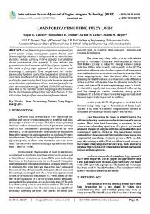
Load forecasting is used to estimate the electrical power demand. In the last few years, several techniques for short- and long- term load forecasting have been discussed, such as Kalman filters, regression algorithms and artificial neural networks [1]. A neural network is a system composed of many simple processing elements operating in parallel whose function is determined by network structure, connection strengths and the processing performed at computing elements or nodes. Artificial neural networks generally consist of three layers: input, hidden and output. Each layer consists of one or more nodes. The inputs to each node in input and hidden layers are multiplied with proper weights and summed together. The weighted composite sum is passed through a proper transfer function whose output is the network output. Typical transfer functions are Sigmoid and Hyperbolic Tangent. For an example of a neural network, see Fig. 1. The layout of the paper is as follows: in section 2 we introduce the proposed method of treating the load prediction problem, section 3 shows the numerical results obtained, and the paper ends with a conclusion.
2
Semi-Parametric Method
When we want to fit a model to data from a power system, we many time have components in the data that are not directly part of the process we want to describe. If a model is fit to the data as it is, then the model parameters will be biased. We would have better estimates of the model parameters if we first remove the unwanted components (nuisance, bias, or non-linear components).
Fig. 1. Artificial Neural Network
This method has been used successfully in the field of spectral estimation in power systems when we analyse the measured signals on power transmission lines [2]. The new method we propose for load forecasting is based on a similar argument to separate the load data into linear and non-linear components. We name this method the Semi-Parametric method for harmonic content identification. We assume that there is an underlying linear part of the load data that could be represented with a sum of n damped exponential functions yL (k) =
n X
Ai ejθi e(j2πfi +di )T k ,
(1)
i=1
where yL (k) is the k − th sample of the linear part of the load signal, Ai is the amplitude, θi is the phase angle, fi is the frequency, di is the damping and T is the sampling period. Since we work only with real signals, the complex exponential functions come in complex conjugate pairs. The equivalent Auto Regressive (AR) model of (1) is given by yL (k) = −
n X
xi yL (k − i) ,
k = n + 1...N ,
(2)
i=1
with model parameters xi , model order n, and N = n + m number of samples in the data set. The model parameters xi and model order n has to be estimated from the data. We propose the following model to separate the linear and non-linear parts [2,3]: yL (k) = y (k) + ∆y (k) , (3) where y (k) is the measured signal sample, ∆y (k) = E [∆y (k)] + � (k) is the residual component consisting of a non-zero time varying mean E [∆y (k)] (nuisance or bias component) and noise � (k). The mean of the residual component is
represented by a Local Polynomial Approximation (LPA) model [4]. yL is then the required linear signal that can be represented with a sum of damped exponentials (1). The LPA model is a moving window approach where a number of samples in the window are used to approximate (filter) one of the samples in the window (usually the first, last or middle sample). The LPA filtering of data was made popular by Savitsky and Golay [5,6]. By substituting eq. (3) in (2) we obtain y (k) + ∆y (k) = −
n X
xi [y (k − i) + ∆y (k − i)] .
(4)
i=1
For n + m samples we have: y (n + 1) + ∆y (n + 1) y (n + 2) + ∆y (n + 2) .. .
= −
y (n + m) + ∆y (n + m)
y (n) + ∆y (n) y (n + 1) + ∆y (n + 1) .. .
··· ···
··· y (n + m − 1) + ∆y (n + m − 1) · · · y (n − 1) + ∆y (n − 1) y (n) + ∆y (n) .. .
y (n + m − 2) + ∆y (n + m − 2) · · · y (1) + ∆y (1) x1 x2 · · · y (2) + ∆y (2) .. . .. .. . . . · · · y (m) + ∆y (m) xn
(5)
In matrix form the model is b + ∆b = −Ax − ∆Ax,
(6)
where b=
y (n + 1) y (n + 2) .. .
,
y (n + m) ∆b =
∆y (n + 1) ∆y (n + 2) .. . ∆y (n + m)
,
· · · y (1) · · · y (2) A= . , .. . .. y (n + m − 1) y (n + m − 2) · · · y (m) ∆y (n) ∆y (n − 1) · · · ∆y (1) ∆y (n + 1) ∆y (n) · · · ∆y (2) ∆A = .. .. .. .. . . . . y (n) y (n + 1) .. .
y (n − 1) y (n) .. .
(7)
.
∆y (n + m − 1) ∆y (n + m − 2) · · · ∆y (m)
(8) The matrix signal model (6) can be rewritten in a different form and represented as � � 1 Ax + b + [∆b ∆A] = 0, (9) x
or Ax + b + D (x) ∆y = 0,
(10)
where the following transformation has been used: � � 1 [∆b ∆A] = D (x) ∆y x
(11)
or
∆y (n) ∆y (n − 1) · · · ∆y (n + 1) ∆y (n + 2) ∆y (n + 1) ∆y (n) ··· .. .. .. .. . . . . ∆y (n + m − 1) ∆y (n + m − 2) · · · ∆y (n + m)
xn · · · x1 1 0 .. . 0
0 ··· . xn · · · x1 1 . . .. .. .. .. .. . . . . . · · · 0 xn · · · x1
1 ∆y (1) x1 ∆y (2) x2 = .. .. . . ∆y (m) xn
0 ∆y (1) .. ∆y (2) . . .. . 0 ∆y (n + m) 1
(12)
If the number of parameters in vector x, (model order n) is not known in advance, the removal of the nuisance component and noise from the signal y (k) is equivalent to estimating the residual ∆y (k) and the model order n while fulfilling constraints (10). To solve the semi-parametric model, the second norm of the noise, plus a penalty term which puts a limit on the size of vector x is minimised. The following optimisation problem should be solved: � � � � 1 µ T 1 µ T 2 T min k�k2 + x x = min (∆y − E [∆y]) (∆y − E [∆y]) + x x x,∆y x,∆y 2 2 2 2 � � 1 µ = min ∆yT W∆y + xT x (13) x,∆y 2 2 subject to the equality constraints Ax + b + D (x) ∆y = 0, where T
W = (I − S) (I − S) ,
(14)
I is the identity matrix, S is the LPA smoothing matrix used to estimate E [∆y (k)] as S∆y, and µ is the Ridge regression factor used to control the size of vector x [7,8]. 2.1
Estimation of the Harmonic Components
The next step is then to calculate the parameters of the harmonic components in eq. (1). We do this as follows [9,10]:
1. The coefficients xi are those of the polynomial H (z) = 1 +
n X
xi z −i ,
(15)
i=1
where z is a complex number z = e(j2πf +d)T .
(16)
By determining the n roots, z i , i = 1, 2, . . . , n , of eq. (15), and using eq. (16) for z, we can calculate the values of the n frequencies and dampings of the harmonic components. It should be noted that we are using complex harmonic exponentials to estimate the input signal’s linear component. However, the signals we measure in practice are real signals of the form
y (k) =
n/2 X
2Ai edi T k cos (2πfi T k + θi ) ,
(17)
i=1
where Ai , θi , fi and di are the same as defined for the complex harmonics in eq. (1). Therefore if we expect to have n2 components in our real signal, there will be n complex harmonic exponentials, and thus will the AR model order be n. The complex harmonic exponentials will then always come in n2 complex conjugate pairs. 2. To determine the n amplitudes Ai and phase angles θi , we substitute the linear component y (k)+∆y (k), and the estimated frequencies and dampings into eq. (1). We obtain an overdetermined system of linear equations of N ×n that can be solved using the least squares method: y (k) + ∆y (k) =
n X
Ai ejθi e(j2πfi +di )T k , k = 1, 2, . . . , N.
(18)
i=1
2.2
Non-Linear Part
The non-linear part (plus the noise), which could represent trends or other nonlinearities in the power system, is then given by yN (k) = y(k) − yL (k) ,
(19)
where yN (k) is the k − th non-linear signal sample and y(k) is the measured load sample. This non-linear part is then used to train a neural network. After the training is complete, the neural network could be used to predict the non-linear part. The linear part is calculated from the signal model (1), which is then added to the non-linear part to obtain the final predicted load values.
3
Numerical Results
For this experiment we used three types of neural networks, namely linear, Backpropagation Multi-layer Perceptron, and a Generalized Regression network [11]. The last network is a kind of Radial Basis network which is often used for function approximation and pattern matching. MATLAB Neural Network toolbox [12] was used for implementation. Before the neural network is trained with the load data, some pre-processing is done on the data. First the data is scaled by the median of the data. Therefore, after prediction, the signal must be descaled by multiplying it again with the median. Then the scaled data is separated into a linear and a non-linear part. The test data, shown in Fig. 2, contained 29 days of load values taken from a town at one hour intervals. This gives a total number of 696 data samples. We
Fig. 2. Load of a Town
removed the last 120 data samples from the training set. These samples would then be used as testing data. Each sample is also classified according to the hour of the day that it was taken, and according to which day. The hours of the day are from one to 24, and the days from one (Monday) to seven (Sunday). The data fed into the network could be constructed as follows: to predict the load of the next hour, load values of the previous hours are used. We can additionally also use the day and hour information. For example, this means that as inputs to the network, we could have k consecutive samples, and two
additional input values representing the hour and day of the predicted k + 1 − th sample. The network will then predict the output of the k + 1 − th sample. We can also call the value of k : a delay of k samples. To evaluate the performance of the different networks, we define a performance index, the Mean Absolute Prediction Error (MAPE): M AP E =
N 1 X |ti − pi | × 100 , N i=1 ti
(20)
where ti is the i − th sample of the true (measured) value of the load, pi is the predicted load value of the network, and N is the total number of predicted samples. For this experiment, the last 24 hours of the 120 removed samples in the load set was used to test the different networks. Different values of delay was used, from five until 96.
Fig. 3. Bad Performance of Method without Separating Data
We also tested the prediction method without splitting the data into linear and non-linear parts, and compared it to the proposed new method. The results of the performance index for each of the networks are shown in Tables 1, 2 and 3. It seems that the method without separating the data into different components performs slightly better than separating the data. In general the method with splitting the data performed well. There were a few occasions where the method
Fig. 4. Performance of Best Network
Table 1. MAPE for Linear Network Separated into Linear / Non-Linear Non-Separated Delay Without day/hour With day/hour Without day/hour With day/hour 5 11.1816 10.8449 6.5760 6.5667 10 9.9194 9.5566 5.9930 5.8607 6.4952 6.5134 16 9.0737 8.8913 2.0441 2.0046 96 2.0096 2.0749
Table 2. MAPE for Multi-layer Perceptron Separated into Linear / Non-Linear Non-Separated Delay Without day/hour With day/hour Without day/hour With day/hour 5 10.0207 6.3053 6.1400 6.7438 10 8.7914 5.6225 5.7735 5.1611 16 8.5937 6.6710 5.8434 30.5284
Fig. 5. Performance of Best Network for Splitting the Data
Table 3. MAPE for Generalized Regression Network Separated into Linear / Non-Linear Non-Separated Delay Without day/hour With day/hour Without day/hour With day/hour 5 13.3721 5.1269 11.1726 4.6823 11.4758 4.5819 10 13.2500 5.1501 16 13.0706 4.7016 11.8720 4.2966 96 8.3921 6.5287 7.6266 5.7553
without splitting the data had very bad performance, eg. Multi-Layer Perceptron with delay 16, as can be seen in Fig. 3. The best network was without splitting the data, delay of 96. This is shown in Fig. 4. The best results for splitting the data is the linear network without day and hour information, delay of 96. This is shown in Fig. 5.
4
Conclusion
The Semi-Parametric method for separating the electric load into a linear and non-linear part was introduced. A neural network was then used to do load forecasting based only on the non-linear part of the load. Afterwards the linear part was added to the predicted non-linear part of the neural network. We compared this method to the usual method without splitting the data. On average the method without splitting the data gave slightly better results, but there were occasions where this method produced very bad networks, whereas the newly introduced method generally performed well.
References 1. Bitzer, B., Rösser, F.: Intelligent Load Forecasting for Electrical Power System on Crete. In: UPEC 97 Universities Power Engineering Conference, UMIST-University of Manchester (1997) 2. Zivanovic, R.: Analysis of Recorded Transients on 765kV Lines with Shunt Reactors. In: Power Tech2005 Conference, St. Petersburg, Russia (2005) 3. Zivanovic, R., Schegner, P., Seifert, O., Pilz, G.: Identification of the ResonantGrounded System Parameters by Evaluating Fault Measurement Records. IEEE Transactions on Power Delivery 19 (2004) 1085–1090 4. Jordaan, J., Zivanovic, R.: Time-varying Phasor Estimation in Power Systems by Using a Non-quadratic Criterium. Transactions of the South African Institute of Electrical Engineers (SAIEE) 95 (2004) 35–41 ERRATA: Vol. 94, No. 3, p.171-172, September 2004. 5. Gorry, P.: General Least-Squares Smoothing and Differentiation by the Convolution (Savitzky-Golay) Method. Analytical Chemistry 62 (1990) 570–573 6. Bialkowski, S.: Generalized Digital Smoothing Filters Made Easy by Matrix Calculations. Analytical Chemistry 61 (1989) 1308–1310 7. Draper, N., Smith, H.: Applied Regression Analysis. Second edn. John Wiley & Sons (1981) 8. Tibshirani, R.: Regression Shrinkage and Selection via the Lasso. Journal of the Royal Society. Series B (Methodological) 58 (1996) 267–288 9. Casar-Corredera, J., Alcásar-Fernándes, J., Hernándes-Gómez, L.: On 2-D Prony Methods. IEEE CH2118-8/85/0000-0796 $1.00 (1985) 796–799 10. Zivanovic, R., Schegner, P.: Pre-filtering Improves Prony Analysis of Disturbance Records. In: Eighth International Conference on Developments in Power System Protection, Amsterdam, The Netherlands (2004) 11. Wasserman, P.: Advanced Methods in Neural Computing. Van Nostrand Reinhold, New York (1993) 12. Mathworks: MATLAB Documentation - Neural Network Toolbox. Version 6.5.0.180913a Release 13 edn. Mathworks Inc., Natick, MA (2002)