http://wjst.wu.ac.th
Applied Mathematics
A New Efficient Algorithm to Solve Non-Linear Fractional Ito Coupled System and Its Approximate Solution Sunil KUMAR Department of Mathematics, National Institute of Technology, Jamshedpur, Jharkhand 831014, India (Corresponding author’s e-mail:
[email protected],
[email protected]) Received: 19 January 2013, Revised: 17 October 2014, Accepted: 31 October 2014
Abstract The aim of the present article is to obtain the approximate analytical solution of time fractional Ito coupled equations by using the homotopy perturbation method. The fractional derivatives are described in the Caputo sense. The highlight of the paper is error analysis between the exact solutions and approximate solutions which shows that our approximate solutions converge very rapidly to the exact solutions. The method gives analytical solution in the form of a convergent series with easily computable components, requiring no linearization or small perturbation. The results reveal that the proposed method is very effective and simple. Keywords: Ito coupled system, fractional derivative, Caputo derivatives, approximate solution, fractional Brownian motion
Introduction Nonlinear partial differential equations have many applications in various fields of science and engineering such as fluid mechanics, thermodynamics, mass and heat transfer, micro electromechanics etc. It is difficult to handle the nonlinear part of these equations. Construction of the exact and explicit solutions of nonlinear partial differential equations is very important in mathematical sciences and it is one of the most stimulating and particularly active areas of the research. It is well known that all nonlinear partial differential equations can be separated into parts: the integrable partial differential equations and non-integrable ones. Fractional differential equations have received more attention in recent years. During the past few years, there has been a growing interest in the field of fractional derivatives. The main reason consists in the fact that the theory of derivatives of fractional (non-integer) order stimulates considerable interest in the areas of mathematics, physics and engineering. Many physical phenomena [1-5] can be modelled by fractional differential equations which have diverse applications in various physical processes such as acoustics, electromagnetism, control theory, robotics, viscoelastic materials, diffusion, edge detection, turbulence, signal processing, anomalous diffusion and fractured media. In this paper, we will use the homotopy perturbation method (HPM) to study a time fractional Ito coupled system. The homotopy perturbation method was first proposed by the Chinese mathematician He [6-8]. In this method the solution is considered as the summation of an infinite series which usually converges rapidly to the exact solutions. The essential idea of this method is to introduce a homotopy parameter, say p , which takes values from 0 to 1, when p 0, the system of equations usually reduces to a sufficiently simplified form, which normally admits a rather simple solution. As p gradually increases to 1, the system goes through a sequence of deformations, the solution for each of which is close to that of the previous stage of deformation. Eventually at p 1, the system takes the original form of the equation and the final stage of deformation gives the desired solution. The method was successfully applied to the
Walailak J Sci & Tech 2014; 11(12): 1057-1067.
A New Efficient Algorithm to Solve Non-Linear Fractional Ito Coupled System http://wjst.wu.ac.th
Sunil KUMAR
space-time fractional advection-dispersion equation by Yildirim and Kocak [9], fractional ZakharovKuznetsov equations by Yildirim and Gulkanat [10], Fokker Planck equation by Yildirim [11], fractional modified Kdv equation by Abdulaziz et al. [12], inversion of the Abel integral equation by Kumar and Singh [13], the fractional Riccati equation by Odibat and Momani [14], the fractional Kdv equation by Wang [15], time-fraction generalized Hirota-Satsuma coupled KdV equation by Ganji et al. [16], multiorder time fractional differential equations by Golbabai and Sayevand [17], explicit analytical solutions of the generalized Burger and Burger-Fisher equations by Rashidi et al. [18], 2 dimensional viscous flow in the extrusion process by Rashidi and Ganji [19], nonlinear coupled equations by Chen and An [20], and a one phase inverse Stefan problem by Slota [21]. Recently, many experts have paid great attention to the construction of solutions of the Ito coupled as symmetry analysis of an integrable Ito coupled system by Zedan [22], numerical solutions for Ito coupled system by Kawala [23], numerical solutions for a generalized Ito system by Zedan and Aidrous [24], double periodic solutions for the generalized Ito system by Zhao et al. [25], Hamiltonian structure for Ito system by Liu [26], invariant for a Ito system by Samoilenko et al. [27], the proposed relation between oHS and Ito systems by Karasu [28], Ito type coupled Kdv equations by Xu and Shu [29], the integrability of a generalized Ito system by Ayse et al. [30], the Hirota-Satsuma coupled KdV equation and a coupled Ito system by Tam et al. [31]. This paper is committed to the study of a time fractional Ito system by using the HPM. Using the appropriate initial conditions, the approximate analytical solutions for different fractional Brownian motions and also for standard motion are obtained. The variation on the approximate solutions is depicted graphically while error analysis shows the accuracy of the approximate analytical solutions. Basic definitions of fractional calculus In this section, we first give the definitions of fractional order integration and fractional order differentiation. For the concept the fractional derivative, we will adopt Caputo’s definition which is a modification of the Riemann Liouville definition and has the advantage of dealing properly with initial value problem. Definition 1 A real function f (t ), t 0 is said to be in the space C , R if there exists a real number p , such that f (t ) t p f 1 (t ) where f 1 (t ) C (0, ) and it is said to be in the space C n if and only if f
(n)
C , n N .
Definition 2 The Riemann-Liouville fractional integral
J
t
operator of order of a function
f C , 1 is defined as; 1 1 t J t f (t ) ( ) 0(t ) f ( )d , ( 0, t 0), J 0 f (t ) f (t ). t
(1)
where (.) is the well-known Gamma function. Some of the properties of the operator ( j t ), can be found in [1-5], we mention only the following. For f C , 1, , 0 and
1 :
(1)
J t J t f (t ) J t f (t ),
(2)
( 2)
J J f (t) J J f (t),
(3)
1058
t t
t t
Walailak J Sci & Tech 2014; 11(12)
A New Efficient Algorithm to Solve Non-Linear Fractional Ito Coupled System http://wjst.wu.ac.th
(3)
( 1) t . ( 1)
J t t
Sunil KUMAR
(4)
The Riemann-Liouville derivative has certain disadvantages when trying to model real world phenomena with fractional differential equations. Therefore, we shall introduce a modified fractional differential operator Dt proposed by Caputo in his work in the theory of viscoelasticity [32].
Definition 3 The fractional derivative Dt of f (t ) in the Caputo sense is defined as;
Dt f (t )
t 1 f ( m ) ( ) d , (m ) 0 (t ) 1m
(5)
where m 1 m, m N , t 0, f C m1 . The following are 2 basic properties of Caputo’s fractional derivative: Lemma 1 If
m 1 m, m N and f C n , 1, then
( Dt J t ) f (t ) f (t ), i m 1 i t ( J t Dt ) f (t ) f (t ) f (0 ) , i! i 0
(6)
Illustrative examples In this section, we discuss the implementation of our proposed algorithm and investigate its accuracy by applying the HPM. The simplicity and accuracy of the proposed method is illustrated through the following numerical examples. Example 1 We consider the time fractional nonlinear Ito coupled system as [22];
Dt u Dx v, 3 Dt v 2( Dx v 3uDx v 3vDx u ) 12wD x w, D w D 3 w 3uD w, x x t with initial conditions u( x,0) nonlinear
u( x, t )
Ito
coupled
0 1, 0 1,
(7)
0 1,
ax a2 x2 and w( x,0) 0. The exact solution of the , v( x,0) 3c 2c 2 1 system (7) for are given as
ax a2 x2 and w( x,0) 0. , v ( x, t ) 3(3at c) 2(3at c) 2
We construct the homotopy which satisfies the;
Walailak J Sci & Tech 2014; 11(12)
1059
A New Efficient Algorithm to Solve Non-Linear Fractional Ito Coupled System http://wjst.wu.ac.th
Sunil KUMAR
Dt u Dx v , 3 Dt v 2( Dx v 3uDx v 3vDx u ) 12 wD x w , D w D 3 w 3uD w , x x t
(8)
and assume the solution of the time fractional Ito coupled system (7) to be in the following form; N
u( x, t ) lim i ui ( x, t ), N
i 0
N
v( x, t ) lim i vi ( x, t ), N
i 0
N
w( x, t ) lim i wi ( x, t ). N
(9)
i 0
where ui ( x, t ), vi ( x, t ), wi ( x, t ), i 0,1,2,3,..., are the functions to be determined. We use the following iterative scheme to evaluate ui ( x, t ), vi ( x, t ), wi ( x, t ). Substituting Eq. (8) into Eq. (9) and equating the coefficients of like powers of we get a system of differential equations. This system of differential equations can be easily solved by applying the operator J t to obtain the various components
un ( x, t ), v n ( x, t ) and wn ( x , t ), thus enabling the series solution to be entirely determined. The first few components of the homotopy perturbation solutions for the Eq. (9) are given as follows;
u0 ( x, t ) u( x,0) u1 ( x, t )
u2 ( x, t )
a2 x t , c 2 ( 1)
v0 ( x, t ) v( x,0) v1 ( x, t )
a2 x2 , 2c 2
w0 ( x, t ) w( x,0) 0,
3a 3 x 2 t , c 3 ( 1)
w1 ( x, t ) 0,
6a 3 x t 9a 4 x 2 t 18a 4 x 2 t 2 , v ( x , t ) , w2 ( x, t ) 0, 2 c 3 ( 1) c 4 ( 1) c 4 (2 1)
u3 ( x , t )
v 3 ( x, t )
ax , 3c
18a 4 x t 2 36a 4 x t 2 , c 4 ( 2 1) c 4 ( 2 1)
54a 5 x 2 c5
2t 3 2t 2 ( 1) t 2 , (3 1) ( 2 1) ( 1)( 1) ( 2 1)
w3 ( x, t ) 0,
and so on. In the same manner the rest of the components can be obtained by the homotopy perturbation solution. Thus the solution u ( x, t ), v ( x , t ) and w( x , t ) of Eq. (7) are obtained by; 8
u~( x, t ) un ( x, t ), n 0
8
v~( x, t ) vn ( x, t ), n 0
8
~ ( x, t ) w ( x, t ) w n
(10)
n 0
The series solution converges very rapidly. The rapid convergence means only a few terms are required to get an analytical function. The simplicity and accuracy of the proposed method is illustrated by computing the absolute errors E u8 ( x, t ) | u(x, t) - u~(x, t) |, E v8 ( x, t ) | v (x, t) - v~(x, t) | where
1060
Walailak J Sci & Tech 2014; 11(12)
A New Efficient Algorithm to Solve Non-Linear Fractional Ito Coupled System http://wjst.wu.ac.th
Sunil KUMAR
~ ( x, t ), v~ ( x, t ) are approximate a 1, c 9, and u ( x, t ), v ( x, t ) are exact solutions and u solutions of (7) obtained by truncating the respective solution series (9) at level N 8. Figure 1 represents the absolute errors between the exact solutions and approximate solutions which shows that ~ ( x, t ) and v~ ( x, t ) converge to the exact solution very rapidly. our approximate solutions u
a
b
Figure 1 The absolute errors E u8 ( x, t ) and E v8 ( x, t ) at a 1 and c 9.
0.0035 0.036
a 1 0. 9
0.032
b
0.0045
0.9 1
v
u
0.034
0.0050
0.8 0.7
0.030
0.7 0.8
0.0040
0.0055
0.028
0.0060 0.0
0.2
0.4
0.6
0.8
1.0
0.0
0.2
t
0.4
0.6
0.8
1.0
t
~ ( x, t ) and v~ ( x , t ) at a 1, c 9. Figure 2 The approximate solution u
The error analysis is depicted in Figure 1 and we can see that a very satisfactory approximate solution of the system with high accuracy is obtained by truncating the HPM solution series at level N 8. Figure 2 shows the behavior of the approximate solutions for different fractional Brownian motions 0.7, 0.8, 0.9 and standard motions 1 when x is constant and time t is
~ ( x , t ) and v~ ( x , t ) with respect to t at x 1 are depicted in Figure 2. It is varying. The variation of u seen from the Figure 2a that the approximate solution u~ ( x, t ) decreases with an increase in t for all
1 at a 1, c 9. Similarly from ~ Figure 2b, it can be seen that the approximate solution v ( x , t ) increases with an increase in t for all values of 0.70, 0.80, 0.90 and for the standard case 1 at a 1, c 9. In this example, values of 0.70, 0.80, 0.90 and for the standard case
Walailak J Sci & Tech 2014; 11(12)
1061
A New Efficient Algorithm to Solve Non-Linear Fractional Ito Coupled System http://wjst.wu.ac.th
Sunil KUMAR
during the numerical computation only 8th order terms of the series solution are considered. The accuracy of the result can be improved by introducing more terms of the approximate solutions. Example 2 We consider the following time fractional nonlinear generalized Ito coupled system as [24,30];
Dt u D x v, 3 Dt v 2 D x v 6 D x (uv ) 6 D x ( wp ), 3 Dt w D x w 3uDx w, D p D 3 p 3uD p, x x t
0 1, 0 1,
(11)
0 1, 0 1,
with initial conditions;
u ( x,0) r1 2 2 tanh 2 ( x), w( x,0) r3 f1 tanh( x),
v( x,0) r2 b2 tanh 2 ( x),
(12)
p ( x,0) t 0 t1 tanh( x).
(13)
The exact solution of the nonlinear generalized Ito coupled system are given as;
b t u ( x, t ) r1 2 2 tanh 2 x 2 2 , 2
b t v( x, t ) r2 b2 tanh 2 x 2 2 , 2
(14)
b t w( x, t ) r3 f1 tanh x 2 2 , 2
b t p( x, t ) t0 t1 tanh x 2 2 . 2
(15)
Here, all the result can be verified through substitution
r3
r1
b22 4 f1t1 2 8b2 4 b2 4 4 r , , 2 8 4 6 2
f1t0 . Where , b2 , t0 , t1 and f 1 are arbitrary constants. t1
We construct the homotopy which satisfies the;
Dt u D x v , 3 Dt v 2 D x v 6 D x (uv ) 6 D x ( wp ) , 3 Dt w D x w 3uDx w , D p D 3 p 3uD p , x x t
0 1, 0 1,
(16)
0 1, 0 1,
We seek the solutions of (11) in the following form; N
u( x, t ) lim i ui ( x, t ), N
1062
i 0
N
v( x, t ) lim i vi ( x, t ), N
Walailak J Sci & Tech 2014; 11(12)
i 0
(17)
A New Efficient Algorithm to Solve Non-Linear Fractional Ito Coupled System http://wjst.wu.ac.th N
N
p( x, t ) lim i pi ( x, t ).
w( x, t ) lim i wi ( x, t ) N
Sunil KUMAR
N
i 0
(18)
i 0
where ui ( x, t ), vi ( x, t ), wi ( x, t ), pi ( x, t ), i 0,1,2,3,..., are the functions to be determined. We use the following iterative scheme to evaluate ui ( x, t ), vi ( x, t ), wi ( x, t ), pi ( x, t ). Substituting Eq. (17) (18) into Eq. (16) and the equating the corresponding power of ;
u0 ( x, t ) u ( x,0) r1 2 2 tanh 2 ( x),
v0 ( x, t ) v( x,0) r2 b2 tanh 2 ( x),
w0 ( x, t ) w( x,0) r3 f1 tanh( x),
u1 ( x, t ) 2 b2 sec h 2 ( x ) tanh( x )
(19)
p0 ( x,0) p ( x,0) t 0 t1 tanh( x).
(20)
t , ( 1)
(21)
(t 1) ,
v1 ( x, t ) 2 sec h 3 ( x )3(t0 f1 t1r3 ) cosh(x ) 23r1b2 3t1 f1 2(3r2 4b2 ) 2
w1 ( x, t ) f1 (3r1 2 2 ) sec h 2 ( x )
p1 ( x, t ) t1 (3r1 2 2 ) sec h 2 ( x )
t , ( 1)
(22)
(23)
t , ( 1)
(24)
and so on. Proceeding in the same manner, the rest of the components un ( x, t ), v n ( x, t ), wn ( x, t ) and
pn ( x, t ) can be obtained and the series solutions are thus entirely determined. Finally, we approximate the analytical solutions u ( x, t ), v ( x, t ), w( x, t ) and p ( x, t ) by truncating the series at level n 3 as; 3
3
v( x, t ) vi ( x, t ),
u( x, t ) ui ( x, t ), i 0
3
3
p( x, t ) pi ( x, t ).
w( x, t ) wi ( x, t ) i 0
Here,
the
accuracy
(25)
i 0
(26)
i 0
of
the
HPM
is
illustrated
by
computing
the
absolute
Eu3 ( x, t ) | u(x, t) - u~(x, t) |, ~(x, t) |, E ( x, t ) | p(x, t) - ~p (x, t) | E v3 ( x, t ) | v (x, t) - v~(x, t) |, E w3 ( x, t ) | w(x, t) - w p3
for
errors
the
constants value of 0.5, f 1 0.6, b2 0.03, t 0 0.4, t1 0.1 and for the standard generalized Ito system i.e. for 1, where u ( x, t ), v ( x, t ), w( x, t ), p ( x, t ) are exact solutions and
Walailak J Sci & Tech 2014; 11(12)
1063
A New Efficient Algorithm to Solve Non-Linear Fractional Ito Coupled System http://wjst.wu.ac.th
Sunil KUMAR
~ ( x, t ), ~ p ( x, t ) are approximate solutions of (11) obtained by truncating the u~( x, t ), v~( x, t ), w respective solutions series (17) - (18). We only consider 3 terms in evaluating the approximate solutions of a generalized Ito system. It achieves a high level of accuracy.
a
b
Figure 3 The absolute errors Eu3 ( x, t ) and E v3 ( x, t ) for a standard generalized Ito system
1 at 0.5, f1 0.6, b2 0.03, t0 0.4, t1 0.1.
a
b
Figure 4 The absolute errors E w3 ( x, t ) and E p3 ( x, t ) for a standard generalized Ito system
1 at 0.5, f1 0.6, b2 0.03, t0 0.4, t1 0.1.
Figures 3 - 4 show the absolute errors between the exact and approximate solutions obtained by the proposed method for values of 0.5, f 1 0.6, b2 0.03, t 0 0.4, t1 0.1 and for the standard
generalized Ito system i.e. for 1. From Figures 3 - 4, it is seen that our approximate solutions obtained by the HPM converge very rapidly to the exact solutions in only the 3rd order approximations i.e. approximate solutions are very near to the exact solutions. It achieves a high level of accuracy. In this example, only the 3rd order term of the series solution is considered. The accuracy of the result can be improved by introducing more terms of the approximate solutions.
1064
Walailak J Sci & Tech 2014; 11(12)
A New Efficient Algorithm to Solve Non-Linear Fractional Ito Coupled System http://wjst.wu.ac.th
0.6 0.4
1
0.130
0.12
Approximate Solution v x, t
Approximate Solution u x, t
0.14
0.10
0 .8 0.08
a
0.06
b
0.135 0.140 0.145
0.8 1
0.150
0.6 0.4
0.155
0.04 0.160
1.0
0.5
0.0
Sunil KUMAR
0.5
1.0
2
1
0
x
1
2
x
~ ( x , t ) and v~ ( x, t ) for different values of and respectively Figure 5 The approximate solutions u when 0.5, f 1 0.6, b2 0.03, t 0 0.4, t1 0.1 at t 1.
0.4 0.6
Approximate Solution w x, t
a 2.2
0.4 0.6
Approximate Solution p x, t
2.0
0.8 1
2.4
2.6
0.35
0.4 0.6
b
0.40
0.45
2.8 2
1
0
1
2
2
x
1
0
1
2
x
~ ( x, t ) and ~ Figure 6 The approximate solutions w p ( x , t ) for different value of and respectively when 0.5, f 1 0.6, b2 0.03, t 0 0.4, t1 0.1 at t 1. The fractional solutions
evaluation results for the approximate solutions are depicted in Figures 5 - 6 for different Brownian motions and standard motions. Figures 5 - 6 show the variation of the approximate ~( x, t ), ~ u~( x, t ), v~( x, t ), w p ( x, t ) for different value , , , vs. x at t 1 and for the
constants value of 0.5, f 1 0.6, b2 0.03, t 0 0.4, t1 0.1. It is seen from the Figure 5a that the approximate solution u~ ( x, t ) increases for the value of x 0 and decreases for the value of x 0 at different value of 0.4, 0.6, 0.8, 1 vs. x. Similarly from Figure 5b, it can be seen that the approximate
x 0 and increasing for the value x 0 at different values of 0.4, 0.6, 0.8, 1 with an increases in x. From Figure 6, we ~ ( x, t ) are strictly increasing and ~p ( x, t ) is strictly decreasing can see that the approximate solutions w with an increases in x at 0.5, f1 0.6, b2 0.03, t 0 0.4, t1 0.1. solution v~ ( x , t ) has the opposite behavior i.e. v~ ( x , t ) is decreasing for the value of
Walailak J Sci & Tech 2014; 11(12)
1065
A New Efficient Algorithm to Solve Non-Linear Fractional Ito Coupled System http://wjst.wu.ac.th
Sunil KUMAR
Conclusions In this paper, the approximate solutions of the fractional order Ito system are obtained by employing the homotopy perturbation method. The beauty of the paper is error analysis between the exact solutions and approximate solutions. We demonstrate that our approximate solutions are very near to the exact solutions despite less computational work for both examples. The results show that the homotopy perturbation method is a powerful and efficient technique in finding exact and approximate solutions for a system of nonlinear partial differential equations of fractional order. Acknowledgement The author is very grateful to the referees for carefully reading the paper and for their comments and suggestions which have improved the paper. The author is highly grateful to the Department of Mathematics, National Institute of Technology, Jamshedpur, India for the provision of some excellent facilities and research environment. References [1] [2] [3] [4] [5] [6] [7] [8] [9] [10] [11] [12] [13] [14] [15] [16]
[17] [18]
1066
KB Oldham and J Spanier. The Fractional Calculus. Academic Press, New York, 1974. KS Miller and B Ross. An Introduction to the Fractional Calculus and Fractional Differential Equations. Johan Willey and Sons, New York, 2003. I Podlubny. Fractional Differential Equations Calculus. Academic Press, New York, 1999. AA Kilbas, HM Srivastava and JJ Trujillo. Theory and Applications of Fractional Differential Equations. Elsevier, Amsterdam, 2006. I Podlubny. Geometric and physical interpretation of fractional integration and fractional differentiation. Fract. Calc. Appl. Anal. 2002; 5, 367-86. JH He. Homotopy perturbation technique. Comput. Meth. Appl. Mech. Eng. 1999; 178, 257-62. JH He. Application of homotopy perturbation method to nonlinear wave equations. Chaos Soliton. Fract. 2005; 26, 695-700. JH He. A coupling method of a homotopy technique and a perturbation technique for non-linear problems. Int. J. Nonlinear Mech. 2000; 35, 37-43. A Yildirim and H Kocak. Homotopy perturbation method for solving the space-time fractional Advection-dispersion equation. Adv. Water Resour. 2009; 32, 1711-6. S Kumar, Y Khan and A Yildirim. A mathematical modelling arising in the chemical system and its approximate solution. Asia Pac. J. Chem. Eng. 2012; 7, 835-40. S Kumar, H Kocak and A Yildirim. A fractional model of gas dynamics equation by using Laplace transform. Z. Naturforsch. 2012; 67, 389-96. S Kumar, MP Tripathi and OP Singh. A fractional model of Harry Dym equation and its approximate solution. Ain Shams Eng. J. 2013; 4, 111-5. S Kumar and OP Singh. Inversion of Abel integral equation by homotopy perturbation method. Z. Naturforsch. 2010; 65, 677-82. Z Odibat and S Momani. Modified homotopy perturbation method: Application to quadratic Riccati differential equation of fractional order. Chaos Soliton. Fract. 2008; 36, 167-74. Q Wang. Homotopy perturbation method for fractional K dV equation. Appl. Math. Comput. 2007; 190, 1795-802. ZZ Ganji, DD Ganji and Y Rostamiyan. Solitary wave solutions for a time-fraction Generalized Hirota-Satsuma coupled KdV equation by an analytical technique. Appl. Math. Model. 2009; 33, 3107-13. A Golbabai and K Sayevand. The homotopy perturbation method for multi-order time fractional differential equations. Nonlinear Sci. Lett. A 2010; 1, 147-54. MM Rashidi, DD Ganji and S Dinarvand. Explicit analytical solutions of the generalized Burgers and Burgers-Fisher equations by homotopy perturbation method. Numer. Meth. Part. Differ. Equat. 2009; 25, 409-17.
Walailak J Sci & Tech 2014; 11(12)
A New Efficient Algorithm to Solve Non-Linear Fractional Ito Coupled System http://wjst.wu.ac.th
Sunil KUMAR
[19] MM Rashidi and DD Ganji. Homotopy perturbation combined with Pad’e approximation for solving two dimensional viscous flow in the extrusion process. Int. J. Nonlinear Sci. 2009; 7, 38794. [20] Y Chen and H An. Homotopy perturbation method for a type of nonlinear coupled equations with parameters derivatives. Appl. Math. Comput. 2008; 204, 764-72. [21] D Slota. The application of the homotopy perturbation method to one phase inverse Stefan problem. Int. Comm. Heat Mass Tran. 2010; 37, 587-92. [22] HA Zedan. Symmetry analysis of an Integrable Ito coupled system. Comput. Math. Appl. 2010; 60, 3088-97. [23] AM Kawala. Numerical solutions for Ito coupled system. Acta Appl. Math. 2009; 106, 325-35. [24] HA Zedan and EA Aidrous. Numerical solutions for a generalized Ito system by using Adomian decomposition method. Int. J. Math. Comput. 2009; 4, 9-19. [25] X Zhao, H Zhi and H Zhang. Improved Jacobi function with symbolic computation to construct new double- periodic solutions for the generalized Ito system. Chaos Soliton. Fract. 2006; 28, 112-26. [26] QP Liu. Hamiltonian structure for Ito system. Phys. Lett. A 2000; 277, 31-4. [27] AM Samoilenko, OM Stanzhytskyj and AM Ateiwi. On invariant Tori for a Stochastic Ito system. J. Dynam. Differ. Equat. 2005; 17, 737-58. [28] A Karasu. Comment: On a recently proposed relation between oHS and Ito systems. Phys. Lett. A 1999; 259, 168-70. [29] Y Xu and CW Shu. Local discontinuous Glerkin methods for the Kuramoto-Shivashinsky equations and the Ito type coupled Kdv equations. Comput. Meth. Appl. Mech. Eng. 2006; 195, 3430-47. [30] KK Ayse, K Atalay and SY Sakovich. Integrability of a generalized Ito system: The Painleve test. J. Phys. Soc. Jpn. 2001; 70, 1165-6. [31] HW Tam, WX Ma, XB Hu and DL Wang. The Hirota-Satsuma coupled Kdv equation and a coupled Ito system revisited. J. Phys. Soc. Jpn. 2000; 69, 45-51. [32] Y Luchko and R Gorneflo. The Initial Value Problem for Some Fractional Differential Equations with the Caputo Derivatives. Fachbreich Mathematick und Informatik, Freic Universitat Berlin, Germany, 1998.
Walailak J Sci & Tech 2014; 11(12)
1067