strip spread can be considered as key points towards improved product quality. ... be regarded as a non-linear mapping of the distorted (true, i.e. Eulerian) strip ...
A NEW EULERIAN-LAGRANGIAN HYBRID FINITE ELEMENT METHOD FOR THE NUMERICAL SIMULATION OF STATIONARY ROLLING PROCESSES A. Kainz and G. Finstermann VOEST-ALPINE Industrieanlagenbau GmbH. Rolling Mill Technologies, Dept. RWW 6 Turmstr. 44, P.O.Box 4, A - 4031 Linz, Austria
ABSTRACT For the analysis of the stationary viscoplastic forming processes in hot rolling of steel, a highly efficient new Eulerian-Lagrangian Hybrid Method has been developed. It is based on an intermediate level of description, using an Eulerian coordinate in the longitudinal direction of the strip, whereas in the width and thickness direction Lagrangian coordinates are employed. The formal conversion of this concept is straight forward, leading to an efficient algorithm, where the time is eliminated as an independent variable. This new method differs significantly from the well known and established “Arbitrary Lagrangian Eulerian“ (ALE) Finite Element concepts based on a moving mesh which is independent of the material flow.
1. INTRODUCTION Although the finite element modelling of steady state rolling processes is not new [1,2], the higher and higher demands from customers concerning product quality are the reason, why improved formalisms are of utmost importance to attain a better understanding of the underlying process details. In hot rolling of steel, a precise prediction of the lateral flow and strip spread can be considered as key points towards improved product quality. In the simulation of hot rolling processes, large material deformations and contact phenomena play an important role. Updated Lagrangian formulations are well suited for problems regarding path dependent material properties and free surfaces, but lead to problems with evolving contacts and suffer from numerical problems, when the mesh is distorted heavily. Moreover, explicit time integrations are necessary in steady state simulations as well. Eulerian formulations [3,4] are able to cope with large material deformations, but are less suited for the description of free surfaces. The Eulerian-Lagrangian method introduced here combines the advantages of the Eulerian field representation by elimination of the explicit time dependence and the individual Lagrangian description with a well known reference configuration. It requires a systematic transformation of the stress-, strain- and strain rate tensors, the balance equations and variational principles of continuum mechanics into this reference frame. The basic concept used for the determination of the velocity field is the principle of virtual velocities, generalised such that the hydrostatic pressure in the strip (incompressibility constraint) and the contact pressure between strip and work roll (penetration constraint) are treated as independent field variables in the sense of a
hybrid formulation. A representation of the Eulerian strain rate tensor and of the Cauchy stress tensor in terms of the Eulerian-Lagrangian coordinates turned out to be most efficient. The transformation from the Eulerian to the Eulerian-Lagrangian level of description can therefore be regarded as a non-linear mapping of the distorted (true, i.e. Eulerian) strip geometry on a fictitious intermediate reference system. The main advantage is that this auxiliary configuration remains unchanged, when updates of the geometry are performed. As a resultant advantageous feature, the streamline integration employed for calculating the actual displacement fields of the strip in width and thickness direction turns out to be a simple one-dimensional integral along the Eulerian coordinate in the longitudinal direction. The rheological behaviour of the strip is treated by using rigid-viscoplastic constitutive laws within the frame of Levy-Mises. Special care is taken of the contact modelling between strip and work roll, in which the Coulomb friction law and the Tresca law (“sticking friction“) have been taken into account. The results, obtained by simulations so far, are compared with those from elementary theories (Kármán Siebel, Sims) [5].
2. BASIC CONCEPTS AND THE METHOD OF ANALYSIS The general formalism outlined in this section is based on a mixed coordinate representation. A spatial (Eulerian) coordinate is employed in the strip direction, whereas material (Lagrangian) coordinates are used in the width and thickness directions. The deformation gradient [6], generating the transition between the different reference frames, has a product decomposition of the form (in tensor notation) E L
t F=
E EL
t F
EL L
t F
(1)
The connection between the three different possible levels of description for stationary process simulations can be represented as follows E L
Eulerian (E.) E EL
t F
t F
Eulerian-Lagrangian (E.L.) EL L
t F
Lagrangian (L.)
(Field representation) r x = ( x1 , x2 , x3 ) r d x = ( dx1 , dx2 , dx3 )
(Intermediate level) r z = ( x1 , a 2 , a 3 ) r d z = ( dx1 , da 2 , da 3 )
(Reduced: a1 ≡ 0 )
Spatial coordinates x i
Referential coordinates z i r Time t = t (z )
Material coordinates a i
Time t does not occur
( t , a 2 , a3 ) r d a = (v IN dt , da 2 , da 3 ) Time t
When dealing with steady state simulations, the knowledge of the behaviour of individual particles located inside a moving layer of the strip with infinitesimal thickness suffices to obtain a full description of the process. This leads to a reduced Lagrangian description where the “particle name” component a1 in strip direction has been eliminated. In general, the input velocity vIN can be an arbitrary function of the Lagrangian coordinates a2 and a3. In rolling simulations, however, the strip velocity is constant over all vertical strip cross sections far enough outside the roll gap.
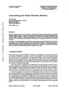
A transformation from the Eulerian (E.) to the Eulerian-Lagrangian (E.L.) level of description can be regarded as a non-linear mapping from the distorted (true) Eulerian geometry to a fictitious intermediate reference system, as depicted in Figure 1. x2
z2 = a2
z1 = x1
x1 Eulerian x 1 - x 2 plane (distorted mesh)
E. L. z1 - z2 plane (rectangular mesh)
Figure 1. Nonlinear mapping on the intermediate Eulerian-Lagrangian reference plane Thet local properties of this transformation are formally described by the deformation gradient E EL F , which is defined by the relation between the infinitesimal coordinate increments t r r d x = ELEF d z . (2) The underlying homomorphism (a unique and invertible relation) is time independent r r r r r ∂x x = x( z ) → ≡ 0 , (3) ∂ t zr leading to a vanishing Eulerian-Lagrangian mesh velocity. The material velocity agrees with the convective velocity describing the material velocity relative to the referential coordinate system. Therefore the formalism treated in this paper is significantly different from simulation methods based on arbitrary Lagrangian-Eulerian (ALE) formulations as outlined e.g. in [7,8]. A systematic evaluation of the concepts based on Eqn. (1) yields the explicit representation ∂ u2 1 + ∂ u2 (4) ∂ z ∂ z 2 3 ∂ u3 1 + ∂ u3 ∂ z2 ∂ z3 r r r with the velocity field components vi ( z ) and u 2 ( z ) and u 3 ( z ) denoting the displacement field components in thickness and width direction, respectively. The displacement vector field is given by the relation r r r r r r r r u ( z ) = x ( z ) − a ( z ) = ( z1 , x2 ( z ) − z 2 , x3 ( z ) − z 3 ) . (5) r The time t = t (z ) is not an independent variable but depends on the E.L. coordinates zi . The operator of the substantial (material) time derivative has a representation of the form d z1 D r ∂ r = v1 ( z ) ↔ dt ( z ) = (time increment). (6) r Dt ∂ z1 v1 ( z ) 1 t v ( zr ) E r F = 2 EL v1 ( z ) v 3 ( zr ) r v1 ( z )
0
0
Therefore, the relations between the displacement and velocity components in thickness and width direction of the strip are given by r r r ∂ ui ( z ) (i = 2, 3) . (7) v i ( z ) = v1 ( z ) ∂ z1 It can be seen from Eqn. (6) that the streamline integration takes a very simple form. It turns out to be a one-dimensional integral along the Eulerian coordinate in strip direction r r r r v( z ) (8) u ( z ) = ∫ dz1 r v1 ( z ) and is used to update the displacement field inside the strip after the velocity field has been determined. The governing equation in weak form is the principle of virtual velocities [9], generalised in the sense of a hybrid formulation t t t t 0 = δπ = ∫∫∫ dV tr σ ′δ D′ + σ M tr δ D′ + δ σ M tr D
[(
)
( )
( )]
r t r r − ∫∫ dS [σ δ v + v δ σ N ] − [TF δ v OUT − TB δ v IN ] V
(9)
SC
TF and TB denote the prescribed specific front and back tensile forces, respectively. The r r independent field variables occurring in Eqn. (9) are the velocity field v (z ) , the mean stress r field σ M (z ) used to satisfy the incompressibility constraint, and the normal contact stress r distribution σ N ( zC ) along the arc of contact to fulfil the penetration constraint between the strip and work roll. Since the normal velocity v N has to be zero along the arc of contact, σ N and v N are treated as conjugate variables. When specifying the longitudinal front and back tensile forces, only one velocity can be prescribed, otherwise the system would be overestimated. For purposes of defining the vector of surface tractions (friction vector), the circumferential velocity of the work roll is specified. The unknown velocity field inside the rolling stock (including the entry and exit velocity of the strip) is then determined by Eqn. (9). Especially for the case of small friction coefficients, an additional stabilisation concept turned out to be beneficial. When neglecting both body forces and effects of inertia, the total sum of all horizontal force components applied to the surface of the strip (including TF and TB) has to vanish. By applying Lagrange parameter techniques, an additional term to the variational expression (9) was added to ensure this “horizontal force constraint“. The friction laws considered so far are the Tresca “sticking“ friction and the Coulomb friction law, where the tangential stress is limited by the yield shear stress. In numerical calculations, regularised frictional laws have to be taken into account to deal with the discontinuity at the neutral point. An arctangent smoothing function as proposed by Kobayashi [1] turns out to be advantageous. t All quantities involved in Eqn. (9) (including the Cauchy stress tensor σ and the rate of t deformation tensor D ) are represented as functions of the E.L. coordinates zi . This avoids the use of the 2nd Piola-Kirchhoff stress tensor and the expressions can be evaluated very efficiently. The discretization and evaluation of Eqn. (9) in the sense of finite element methods [9,10], where the arbitrariness of the virtual variations is utilised, leads to a finite number of coupled nonlinear equations of the form r r r r 0 = δπ ( X ) = δX ⋅F(X) → Fi ( X 1 , X 2 ,... X N ) = 0 (10)
that have to be solved numerically. N denotes the total number of degrees of freedom. The r global solution vector X contains nodal velocity-, mean stress- and normal contact stress components, as is obvious from Eqn. (9). All partial derivatives t ∂ FI KI J = ( N × N stiffness matrix K ) (11) ∂ XJ are calculated analytically. Linear subproblems of the form r r t r r r r F(X) + K(X) ? X = 0 (increment ∆X ) (12) can be treated economically (both with respect to storage requirements and calculation time) by employing sparse nonsymmetric linear equation solvers. Especially such ones based on multifrontal variants of the Gaussian elimination have proved to be very efficient. Special attention should be paid to suitable preconditioners, because otherwise “fill - in effects“ lead to numerical inefficiency. Concerning the nonlinear problem Eqn. (10), a simple iterative Newton-Raphson algorithm did not always converge. Therefore, an implementation of the “dogleg-algorithm“, combined with trust region updates, was performed. The dogleg trajectory is a convex combination of the r r Newton direction v and the scaled steepest descent direction g , as shown in Figure 2. r g C.P. R
r X old
r X new
r r α g+β v
r v
Figure 2. The double dogleg step from r r X old to X new in nonlinear analysis (C.P. denotes the Cauchy point, R is the current radius of the trust region)
The size of the trust region radius R is adjusted according to how well the norm of the system r r r of equations F ( X + ∆X ) is reduced compared with expectations based on local quadratic approximations (S.Q.P.: sequential quadratic programming method). This self-adaptive technique adjusts tolerances and chooses solution approaches automatically to obtain an optimum global solution. Further details are given in [11]. From the global solution of Eqn. (9), the velocity field, the stress and strain rate distributions inside the strip are known. The contact stresses between strip and roll are input parameters for the elastic roll deformation model. To obtain correct results, both the geometry and the plastic strain distribution have to be updated by the streamline method. This leads to an iterative calculation process represented in Figure 3. Summarising the main advantages of the Eulerian-Lagrangian formalism as described above, the following four items should be emphasised: • time independent reference configuration (zero mesh velocity) • the E.L. mesh remains unchanged when updates of the geometry are performed • the streamline integration is a simple integral along the Eulerian coordinate • an undistorted rectangular reference mesh suffices in two-dimensional calculations.
INITIAL ESTIMATES for vi , σ M , σ N , ui (Elementary rolling theory) ui Principle of VIRTUAL VELOCITIES (Geometry is kept fixed) vi , σ M , σ N GEOMETRY UPDATE: • Streamline integration • Work roll surface contour ui
no
Converged ? yes Postprocessing
Figure 3. Global flow chart of the model
3. NUMERICAL RESULTS The general formalism based on the preceding section has been applied to two-dimensional plane strain models and prescribed roll bite geometry, i.e. rigid rolls. Both the Tresca friction law (sticking friction) and the Coulomb law (slipping friction) are taken into account. The rolling process under consideration produces deformation symmetrically with respect to the strip thickness centre line, so that only half of the strip has to be modelled. The deformation was assumed as plane strain and the rolls were idealised as rigid. A typical distorted Eulerian finite element mesh is shown in Figure 4. The corresponding displacement field in thickness direction generating the transition to the undistorted Eulerian-Lagrangian rectangular mesh is given in Figure 5. It should be emphasised that the method of geometric mesh refinement at the roll entry and exit side has proved to be effective. Both in upstream and downstream direction, the mesh has to be extended far enough outside the roll gap to ensure numerical convergence.
27
18
u2 [mm]
x2 [mm]
0
9
-4
-8
Contact surface Symmetry plane
-12
0 -180
-120
-60
0
z1 [mm]
Figure 4. The distorted Eulerian finite element mesh for 2D-flat rolling
60
-180
-120
-60
0
60
z1 [mm]
Figure 5. The corresponding displacement field u2 in thickness direction
11
0
-0.4
9
v2 [m/s]
v1 [m/s]
Contact surface Symmetry plane
7
-0.8 -1.2 -1.6
5 -300
-200
-100
0
Contact surface Symmetry plane
-300
50
-200
-100
0
50
z1 [mm]
z1 [mm]
Figure 7. The same as in figure 6 for the velocity field v2 in the thickness direction
Figure 6. Velocity field component v1 in the strip direction as a function of z1 for several z2 values inside the rolling stock
On account of the variational formalism based on velocity fields, special care is taken of the smoothness properties of the distributions, which can be controlled by proper discretization. In Figures 6 and 7 the velocity components v1 and v2 in strip and thickness direction, respectively, are represented as functions of the Eulerian coordinate z1 for several z2 values inside the strip. As expected, particles at the surface of the strip are strongly accelerated when entering the roll gap and therefore move faster compared to those in the strip symmetry plane. At the neutral zone, the sign of the tangential stress changes and the mid-plane particles become faster compared to those at the surface. This behaviour leads to a different run-time of individual particles through the roll gap. In Fig. 8, the deviation of the run-time of individual particles (characterised by the coordinate z2) from the time of a mid-plane particle is plotted as a function of z1. It can be seen that surface particles are fastest in total, although at the exit side they are the slowest ones. For rolling conditions, where the assumption of homogeneous compression is almost fulfilled, the residual time difference tends to zero because the horizontal velocity is nearly constant over vertical cross-sections. Of special interest is the behaviour near the neutral point. The relative velocity between the strip and the work roll is a significant measure for the magnitude of the neutral zone. In hot rolling conditions with high friction coefficients, the neutral zone is well pronounced and extends to several contact surface elements, where sticking occurs. Such a typical situation is shown in Figure 9 for a friction coefficient µ = 0.5. Relative velocity [m/s]
Run-time dev. [ms]
0 -0.4 -0.8
-1.2 -1.6 -400
Contact surface Symmetry plane -300
-200
-100
0
100
200
z1 [mm]
Figure 8. The deviation of the particle runtime inside the strip from the reference time calculated in the symmetry plane of the strip
1 0 -1 -2 -3 -160
-120
-80
-40
0
z1 [mm]
Figure 9. Relative velocity between work roll and surface of the strip inside the roll gap
Tangential stress [N/mm^2]
Normal stress [N/mm^2]
Lagrange parameter Kármán Siebel
Lagrange parameter extrapolated values z1 [mm]
z1 [mm]
Figure 11. Distribution of the tangential nodal traction for the Tresca friction law
Figure 10. Normal pressure distribution along the arc of contact for the case of a strongly pronounced friction hill
Contact surface Symmetry plane z1 [mm]
Figure 12. Shear stress distribution inside the strip as a function of z1 for several z2 values in the case of Tresca friction
Normal stress [N/mm^2]
Shear stress [N/mm^2]
In Figure 10, the normal contact stress distribution along the arc of contact is depicted as a function of the Eulerian coordinate z1 in strip direction for the Tresca friction law. The calculation is performed both by employing Lagrange parameter techniques and by an extrapolation of the stress values evaluated at the gauss points inside the strip. The results agree extremely well inside the roll gap; only at the entry point (first contact between strip and work roll) small deviations occur. For comparison, the result obtained by solving the Kármán-Siebel differential equation is also given, which is a good approximation of the rolling situation considered. Figure 11 shows the corresponding shear stress distribution along the surface of the strip. Lagrange parameter Karman Siebel
z1 [mm]
Figure 13. Distribution of the normal traction for a slab, where the friction hill parameter is small
The shear stress distribution inside the strip is represented in Figure 12. For the exact solution the shear stresses should become zero at the symmetry plane. However, when dealing with discrete solution methods like finite elements, only an approximation tending to this result for increasing mesh refinement can be expected at all. While in Fig. 10 a well pronounced friction hill occurs, Figure 13 shows the normal contact stress distribution for the case of a small friction hill parameter. Again, the Kármán-Siebel solution is given for comparison. The significant deviation of the finite element results from this solution is due to the breakdown of the assumption of homogeneous deformation.
Plastic strain rate [1/s]
Tangential stress [N/mm^2]
Contact surface
Lagrange parameter extrapolated values
Symmetry plane
z1 [mm]
z1 [mm]
Figure 14. The tangential stress along the arc of contact in the case of Coulomb friction limited by the shear yield stress
Figure 15. Distribution of the plastic strain rate inside the strip as a function of z1 for several z2 values
In Figure 14 the shear stress distribution is shown for the Coulomb friction law (friction coefficient µ = 0.2 ), where the tangential stress is limited by the shear yield stress. As in Fig. 11, the two curves agree satisfactorily on the scale of the figure. The uniaxial plastic strain rate distribution depicted in Figure 15 shows an interesting behaviour at the neutral zone. There the largest strain rates occur at the symmetry plane, whereas everywhere else the situation is reverse. This local effect of almost vanishing plastic compression corresponds to tribologic conditions, where a significant neutral zone occurs (cf. Fig. 9). To conclude this section, a comparison between Eulerian-Lagrangian simulation results and those obtained by solving the Kármán-Siebel differential equation is given in Table I. For small roll gap aspect ratios, defined by the ratio of the mean strip thickness to the contact length hM / LD , both methods are expected to lead to similar results. In this test calculation a strip of steel grade ST37 (low carbon) with a thickness of 2 mm is rolled to a 40% reduction in thickness by a work roll with a radius of 350 mm. Concerning the tribologic aspects the Coulomb friction law (µ=0.3) limited by the shear yield stress is assumed. Except for the mean strain rate that seems to be overestimated by the material flow simulations, the results correspond satisfactorily.
Spec. rolling force [kN/mm] Spec. horizontal force [kN/mm] Spec. rolling torque [kN] Spec. mech. power [kN/s] Neutral point / contact length Forward slip [%] Backward slip [%] Input velocity [m/s] Output velocity [m/s] Mean kfp [N/mm^2] Mean strain-rate [1/s]
Eulerian-Lagrangian 14.65 -0.0015 112.33 4809 0.415 11.53 33.39 4.99 8.36 273.7 292.4
Kármán-Siebel 15.12 0.0023 111.44 4771 0.411 11.22 33.27 5 8.33 267.7 199.3
Table I. Comparison with Kármán-Siebel for the Coulomb friction law and small roll gap aspect ratio hM / LD = 0.088
4. CONCLUSIONS As described above, the novelty of the formalism outlined in this paper is the use of a mixed coordinate reference configuration, which is time independent and remains unchanged when updates of the geometry are performed. In 2D simulations, an undistorted rectangular mesh suffices to obtain satisfactory results. The general formalism has been applied to twodimensional plane strain models and prescribed roll bite geometry, i.e. rigid rolls. Generalisations, including the coupling with elastic roll deformation and further extension to three-dimensional problems are straightforward in principle and in elaboration. The availability of a 3D-simulation tool based on the Eulerian-Lagrangian concepts will enable the accurate determination of the transverse material flow and of strip spread in hot rolling simulations. Besides, the precise prediction of profile, flatness and of profile adjustment ranges is of particular interest. This will be accomplished by coupling the Eulerian-Lagrangian material flow program with the routines predicting roll stack deflection. TABLE OF SYMBOLS xi zi ai ui vi
= Eulerian (E.) coordinates [mm] = Eulerian-Lagrangian (E.L.) coord. [mm] = Lagrangian (L.) coordinates [mm] = Displacement field components [mm] = Velocity field components [m/s]
t E EL F = Deformation gradient (from E.L. to E.) Di j = Rate of deformation tensor [1/s]
σi j
= Cauchy stress components [N/mm^2]
FI = Global stiffness vector K I J = Global stiffness matrix XI σM σN vN t D′ t σ′
= Global solution vector = Mean stress field [N/mm^2] = Normal contact stress [N/mm^2] = Normal velocity [m/s]
t D [1/s] t = Deviator of the tensor σ [N/mm^2] = Deviator of the tensor
REFERENCES 1. Kobayashi S, Oh S, Altan T, ‘Metal forming and the finite-element method’, Oxford University Press, New York, 1989. 2. Montmitonnet P, Buessler P, ‘A review on theoretical analyses of rolling in Europe’, ISIJ International, Vol. 31, No. 6, 1991 3. Karabin M, Smelser R, ‘A quasi three-dimensional analysis of the deformation processing of sheets with applications’, ., Int. J. Mech.Sci., Vol.32, No. 5, 1990 4. Iguchi T, Yarita I, ‘3-dimensional analysis of flat rolling by rigid-plastic FEM considering sticking and slipping frictional boundary’, ISIJ International, Vol. 31, No. 6, 1991 5. Orowan E, ‘The calculation of roll pressure in hot and cold flat rolling’, Proc. Inst. Mech. Engrs., Vol. 150, 1943 6. Betten J, ‘Kontinuumsmechanik’, Springer, 1993. 7. Chenot J, Bellet M, ‘The ALE method for the numerical simulation of material forming processes’, Simulation of Materials Processing, Balkema, Rotterdam, 1995. 8. Liu W, Chang H, Chen J, Belytschko T, ‘Arbitrary Lagrangian-Eulerian Petrov-Galerkin finite elements for nonlinear continua’, Computer Methods in Appl. Mechanics and Engineering, 68, 1986 9. Bathe K, ‘Finite Element Procedures in Engineering Analysis’, Prentice Hall, 1982 10. Zienkiewicz O, Taylor R, ’The finite element method’, Vol. 1 and 2, McGraw-Hill, 1997 11. Dennis J, Schnabel R, ‘Numerical methods for unconstrained optimisation and nonlinear equations’, Prentice Hall, 1983