LMS (RZA-LMS) [2] and the l0-LMS [3], while similar to that of the non-uniform norm constraint LMS (NNCLMS) [6], and smaller than that of the sparsity-aware ...
IEEE COMMUNICATIONS LETTERS, VOL. , NO. , 2015
1
A New l0-LMS Algorithm with Adaptive Zero Attractor Chengcheng Wang, Yonggang Zhang, Member, IEEE, Ye Wei, and Ning Li, Member, IEEE
Abstract— In the l0 -norm constraint least mean square (l0 LMS) algorithm, the zero attractor is an important parameter which balances the trade-off between the convergence rate and steady-state error of the algorithm. However, there is no practically effective choice guideline of this parameter. In addition, the optimal value of this parameter should be time-varying when the measurement noise power varies with time, and a fixed value of the zero attractor is no longer suitable. In this letter, we propose an l0 -LMS algorithm with adaptive zero attractor for applications with time-varying measurement noise signal, where the zero attractor is updated based on the criterion of maximizing the decrease of the transient mean square deviation. Index Terms— l0 -LMS algorithm, adaptive zero attractor, timevarying measurement noise signal, sparse system identification.
I. I NTRODUCTION We consider the applications of sparse system identification where there are only large and zero coefficients in the unknown impulse responses. Such impulse responses are encountered in a number of different applications, for instance, in highdefinition television (HDTV), broadband wireless communications in hilly terrain, underwater acoustic channels and so on [1]. In recent sparsity-aware LMS algorithms, an lp norm like constraint of the tap-weight vector is integrated into the cost function of the classical LMS algorithm [2]–[6] and [7]. A zero-attraction term is thereby added to the update equation of the filter tap-weight vector, which aims to accelerate the identification speed by attracting small coefficients towards zero. However, both the steady-state performance and instantaneous behavior of all these lp norm constraint based algorithms will depend on the selection of the zero attractor, which controls the strength of the zero-attraction term [4], [5]. Moreover, in order to ensure good steady-state mean square performance, the zero attractor should be set according to the power of the measurement noise signal [4], [5]. This makes the parameter settings of these sparsity-aware algorithms with fixed zero attractors even more difficult, especially for applications where the measurement noise signal is time-varying. Manuscript received July 29, 2015; revised September 8, 2015, accepted October 5, 2015. This work was supported by the National Natural Science Foundation of China (grant 61201409 and 61371173), China Postdoctoral Science Foundation (grant 2013M530147 and 2014T70309), Chinese Government Scholarship, Heilongjiang Postdoctoral Fund (grant LBH-Z13052 and LBH-TZ0505) and Fundamental Research Funds for the Central Universities of Harbin Engineering University (grant HEUCFQ20150407). The associate editor coordinating the review of this paper and approving it for publication was P. S. Rossi. (Corresponding author: Yonggang Zhang.) The authors are with the College of Automation, Harbin Engineering University, Harbin, Heilongjiang 150001 China (e-mail: {wangchengcheng, zhangyg, weiye, ningli}@hrbeu.edu.cn).
To solve this problem, in this letter we propose an adaptive strategy to select the zero attractor in the l0 norm constraint LMS (l0 -LMS) algorithm. A theoretically optimal zero attractor is firstly derived for each iteration by maximizing the decrease of transient mean square deviation (MSD) during the convergence process. Then a practically effective update equation for the zero attractor is obtained based on the characteristics of sparsity and the zero-attraction term. Finally, simulation results illustrate that the proposed algorithm is endowed with the ability to adapt to time-varying measurement noise signal, outperforming the existing techniques with fixed zero attractors. Notation: All variables and vectors used in this letter are real for simplicity. We utilize bold fonts to denote vectors, and normal ones to denote scalars. The operator (·)T denotes the transpose of a real vector, sgn(·) is a component-wise sign function, and E{·} represents the statistical expectation. . Moreover, notations | · |, ∥ · ∥1 , ∥ · ∥, and = denote respectively the absolute value, the l1 norm and Euclidean norm of a vector, and a definition. II. P ROBLEM S TATEMENT Consider the following linear regression model: T d(n) = wopt x(n) + v(n)
(1)
with d(n), wopt , x(n), and v(n) denoting the desired signal, the unknown impulse response vector, the input vector, both of size L, and the noise signal. In the l0 -LMS algorithm, the update equation for the tap-weight vector is as follows [3]: w(n + 1) = w(n) + µe(n)x(n) + ρξ0 (w(n))
(2)
where w(n) = [w0 (n), w1 (n), . . . , wL−1 (n)]T is the filter tapweight vector, n is the time index, the parameter µ is the stepsize of the adaptation. The output error e(n) is the difference between the desired signal d(n) and the output signal from the adaptive filter: e(n) = d(n) − wT (n)x(n).
(3)
Moreover, the last term ρξ0 (w(n)) on the right hand side (RHS) of equation (2) denotes the zero-attraction term, where the parameter ρ > 0 is the zero attractor, the term ξ0 (w(n)) is the subgradient of the approximate l0 norm penalty on the tapweight vector, and for each entry 0 ≤ i < L, the subgradient is specified as [3]: { 2 α wi (n) − αsgn(wi (n)), |wi (n)| ≤ 1/α . ξ0 (wi (n)) = 0, elsewhere (4)
2
IEEE COMMUNICATIONS LETTERS, VOL. , NO. , 2015
where positive parameter α > 0 determines the zero-attraction strength and range. Previous study on the zero attractor in the l0 -LMS algorithm shows that from the perspective of steady-state MSD, theoretically optimal zero attractor is positively related to the noise signal power (equation (17) in [5]). As a result, if there is a change in the power of the measurement noise signal, we should reset a value to the zero attractor to obtain a better steady-state performance of the l0 -LMS algorithm. In order to endow the l0 -LMS algorithm with the ability to adapt to time-varying measurement noise signal, we propose the l0 -LMS algorithm with adaptive zero attractor (AZA-l0 LMS) in the following section, based on the criterion of maximizing the decrease of transient MSD. III. P ROPOSED A LGORITHM In this section, we firstly derive the theoretically optimal zero attractor at each iteration by maximizing the decrease of transient MSD during the convergence process. Then we will make a practical approximation of the optimal solution and propose the AZA-l0 -LMS algorithm. Finally, computational complexity is analysed for the proposed algorithm as well as some existing sparsity-aware algorithms. A. Optimal Zero Attractor We intend to find the optimal zero attractor ρopt according to the following cost function: { } . 2 ρopt = minρ E ∥w(n ˜ + 1)∥2 − ∥w(n)∥ ˜ (5) where
. w(n ˜ + 1) = wopt − w(n + 1)
(6)
denotes the deviation from unknown impulse response vector at time n + 1. Different from the derivation in [5], where the optimal zero attractor is defined by minimizing the steady-state MSD, we update the zero attractor on the basis of transient MSD. By setting the zero attractor to the value that contributes to the steepest decrease of the transient MSD, we intend to adjust the parameter adaptively to time-varying measurement noise signal. Meanwhile, this ensures that the zero attractor will converge to the theoretically optimal value that leads to the minimum steady-state MSD of the l0 -LMS { } algorithm in [5]. 2 The term E ∥w(n ˜ + 1)∥2 − ∥w(n)∥ ˜ on the RHS of (5) can be obtained by subtracting both sides of (2) from wopt before taking expectations and some algebra operations, that is { } 2 E ∥w(n ˜ + 1)∥2 − ∥w(n)∥ ˜ { } = ρ2 (n + 1)E ξ0T (w(n))ξ0 (w(n)) { } + 2µρ(n + 1)E e(n)xT (n)ξ0 (w(n)) { T } − 2ρ(n + 1)E w ˜ (n)ξ0 (w(n)) { } + µ2 E e2 (n)xT (n)x(n) { T } − 2µE w ˜ (n)x(n)e(n) (7) Note that by utilizing notation ρ(n + 1), we are indicating that the zero attractor is adaptive, and also deterministic at each time index as we can take it out of the expectation functions.
Take the partial derivatives with respect to ρ(n + 1) on both sides of (7), and set them to zero, then we can obtain the optimal zero attractor at time n + 1: ρopt (n + 1) = { T } { } E w ˜ (n)ξ0 (w(n)) − µE e(n)xT (n)ξ0 (w(n)) { T } E ξ0 (w(n))ξ0 (w(n))
(8)
B. The AZA-l0 -LMS Algorithm In practice, the three expectations on the RHS of (8) can be approximated by their unbiased time averages respectively, namely ψ(n + 1) = βψ(n) + (1 − β)w ˜ T (n)ξ0 (w(n))
(9)
φ(n + 1) = βφ(n) + (1 − β)e(n)x (n)ξ0 (w(n))
(10)
ϕ(n + 1) = βϕ(n) + (1 − β)ξ0T (w(n))ξ0 (w(n))
(11)
T
where the notations ψ(n + 1), φ(n +{1) and ϕ(n + 1) } denote the approximations of the terms E w ˜ T (n)ξ0 (w(n)) , { } { } E e(n)xT (n)ξ0 (w(n)) and E ξ0T (w(n))ξ0 (w(n)) respectively, and initially we select ψ(0) = 0, φ(0) = 0 and ϕ(0) = 0. Moreover, β > 0 is the smoothing parameter and is set very close to unity to apply sufficient time smoothing. Thereby the optimal zero attractor defined in (8) can be approximated to: { ψ(n+1)−µφ(n+1) , if ϕ(n + 1) ̸= 0 ϕ(n+1) ρopt (n + 1) = (12) 0, if ϕ(n + 1) = 0 In the following simulations, we take the result calculated from (12) as a theoretical reference. Remark 1: Note that in the case when the denominator ϕ(n + 1) is zero in equation (12), we can just set ρopt (n + 1) to 0, then the proposed algorithm will behave as the classical LMS algorithm. That is because the term ϕ(n + 1) defined in (11) will be zero if and only if the entries in the tap-weight vector are either zero or greater than the value of 1/α, in which case there is no attraction towards zero on all the coefficients according to the definition in (4). Before we proceed, the following assumption is made for convenience of analysis: Assumption 1: The unknown system impulse response vector only has large coefficients and zero coefficients, with no near-zero coefficients. This assumption matches the observations in many applications, as is indicated in the introduction. We continue to consider the term w ˜ T (n)ξ0 (w(n)) on the RHS of (9), since the deviation vector w(n) ˜ is not available. Based on the definition in (6), we can rewrite the term mentioned above as: T w ˜ T (n)ξ0 (w(n)) = wopt ξ0 (w(n)) − wT (n)ξ0 (w(n)) (13)
where the second term on the RHS is always available at real time. The first term on the RHS of equation (13) can be equivalently written as follows, based on Assumption 1: ∑ ∑ T wopt ξ0 (w(n)) = wopt,i ξ0 (wi (n)) + wopt,i ξ0 (wi (n)) i∈CL
i∈C0
(14)
WANG et al.: A NEW L0 -LMS ALGORITHM WITH ADAPTIVE ZERO ATTRACTOR
LMS RZA−LMS
0
. CL = {i | |wopt,i | > 1/α} , . C0 = {i | wopt,i = 0}
l0−LMS, ρ = 2.5*10−4
−10
l0−LMS, ρ = ρopt
Transient MSD(dB)
where Large Coefficients: Zero Coefficients:
3
−20
NNCLMS SA−ALT−LMS AZA−l0−LMS (practical)
−30
AZA−l0−LMS (theoretical)
−40
w ˜ T (n)ξ0 (w(n)) ≈ −wT (n)ξ0 (w(n))
(15)
then equation (9) is simplified as: ψ ′ (n + 1) = βψ ′ (n) − (1 − β)wT (n)ξ0 (w(n))
TABLE I T HE P ROPOSED AZA-l0 -LMS A LGORITHM Start with {w(0) = 0L , ψ ′ (0) = 0, φ(0) = 0, ϕ(0) = 0, ρ(0) = 0}. Given µ, α, β, for each time n ≥ 0, repeat: (i) Calculate error through equation (3) (ii) Calculate subgradient vector ξ0 (w(n)) through equation (4) (iii) Update terms ψ ′ (n+1), φ(n+1) and ϕ(n+1) following equations (16), (10) and (11) respectively (iv) Update zero { attractor ψ ′ (n+1)−µφ(n+1) , ϕ(n+1)
if ϕ(n + 1) ̸= 0 0, if ϕ(n + 1) = 0 (v) Update tap-weight vector w(n + 1) = w(n) + µe(n)x(n) + ρ(n + 1)ξ0 (w(n))
C. Computational Complexity In this section, computational complexity of the proposed AZA-l0 -LMS algorithm and some existing sparsity-aware LMS algorithms is compared in Table II, in terms of arithmetic operations, comparisons, and memory requirements. As shown in Table II, the amount of computations of the proposed algorithm is 2/3 more than that of the reweighted zero-attracting LMS (RZA-LMS) [2] and the l0 -LMS [3], while similar to that of the non-uniform norm constraint LMS (NNCLMS) [6], and smaller than that of the sparsity-aware alternating optimization LMS (SA-ALT-LMS) [7]. TABLE II C OMPUTATIONAL C OMPLEXITY OF A LGORITHMS Algorithm LMS RZA-LMS [2] l0 -LMS [3] NNCLMS [6] SA-ALT-LMS [7] AZA-l0 -LMS
Computational Complexity (2L)ad+(2L+1)mult+(L)memo (4L)ad+(5L+1)mult+(L)memo (4L)ad+(5L+1)mult+(L)comp+(L)memo (7L-1)ad+(7L+2)mult+(L)memo (7L)ad+(11L+1)mult+(2L)comp+(2L)memo (7L+1)ad+(8L+10)mult+(L)comp+(L+3)memo
Transient MSE(dB)
0
500
1000
1500
2000
2500 −32
0
−34
−10
−36
−20
2500
−30
2600
0
500
1000
1500
2000
2500
0
500
1000
1500 Iterations
2000
2500
2700
−30 −35 −40 −45
Fig. 1. Transient MSDs (top), and MSEs (middle) of LMS, RZA-LMS, l0 LMS, NNCLMS, SA-ALT-LMS and AZA-l0 -LMS algorithms and transient zero attractors (bottom) of l0 -LMS and AZA-l0 -LMS algorithms in a high sparsity case.
(16)
where we use ψ ′ (n + 1) to distinguish from ψ(n + 1) defined in (9). As is shown in the subsequent simulation results, the approximation in (15) is reasonable due to the quick convergence rate of the large tap-weights. The proposed AZA-l0 -LMS algorithm is summarized in Table I, where 0L represents a zero vector of size L.
ρ(n + 1) =
−50
ρ(n) (dB)
both follow the definitions in [5]. Thus the second term on the RHS of (14) goes to zero by definition. Furthermore, the first term on the RHS of (14) will disappear as well after the large tap-weights converge to sufficiently large values that are larger than the value of 1/α, according to the definition in (4). Consequently, equation (13) can be approximated to:
IV. S IMULATION R ESULTS In this section, we will test the performance of the proposed AZA-l0 -LMS algorithm when the measurement noise signal power varies abruptly. The standard LMS algorithm, RZALMS algorithm [2], the l0 -LMS algorithms with fixed zero attractor [3] and theoretically optimal zero attractor [5], the NNCLMS [6], and the SA-ALT-LMS [7] are also tested for comparison. The first experiment is to test the performance of the AZAl0 -LMS algorithm in a high sparsity case. The setup of the simulation is as follows. The unknown system coefficient vector has a length of 64, and we randomly set 2 of them to 1, while the others to 0. The exciting and noise signals are drawn from uncorrelated zero-mean white Gaussian sequences. The exciting signal power is set to 1, while the noise signal power is scaled to make the signal-to-noise ratio (SNR) change from 15dB, to 0dB at the 1000th time index, and finally to 40dB at the 1500th time index. We set step-size µ = 0.01 in all the tested algorithms, and the parameter ε = 20 in the RZA-LMS, and α = 10 in all the other algorithms; Moreover, in the RZALMS and NNCLMS, we set zero attractor ρ = 2.5 × 10⁻³ , while ρ = 2.5 × 10⁻⁴ in the l0 -LMS; In the SA-ALTLMS, we set η = 8 × 10⁻³ , λ = 0.03, τ = 0.03; In the proposed algorithm, we set the smoothing parameter β = 0.99. The above parameters are set to ensure similar steady-state performance in all the strategies when SNR is 15dB. Fig.1 shows the evolution curves for these tested schemes in a high sparsity case, and the results are averaged over 100 independent experiments. As can be seen from Fig.1 that initially when the SNR is set to 15dB, the tested sparsity-aware LMS algorithms with pre-determined zero attractors have similar performance to the proposed AZA-l0 -LMS algorithm, outperforming the standard LMS algorithm. However, as the SNR drops to 0dB, performance of the sparsity-aware LMS algorithms with fixed zero attractors deteriorates, resulting from deficient zeroattraction strength for small tap-weights. When the SNR goes up to 40dB, the best steady-state performance is obtained in the proposed AZA-l0 -LMS algorithm, as a result of zero attractor adapting to time-varying measurement noise signal power. Moreover, it is also clear to see that the zero attractor
4
IEEE COMMUNICATIONS LETTERS, VOL. , NO. , 2015
NNCLMS SA−ALT−LMS AZA−l0−LMS (practical)
Transient MSD(dB)
l0−LMS, ρ = ρopt
−20 −30
Transient MSE(dB)
−5
l0−LMS, ρ = 2*10
−10
0
500
1000
1500
2000
2500
0
−42
−10
−44 −8
−20
−46 −48 2650
−10
−30
−12
−40
1450 0 ρ(n) (dB)
0
500
1000
1500
2000
10 Transient MSE(dB)
AZA−l0−LMS (theoretical) −40
500
1000
500
1000
1500
1550 1500
2700
2750
2800
1600 2000
2500
2000
2500
−40
−50
2500
−45 −50 −55 −60
−44
0
−10
1500 Iterations
−46
−20 −30
−48 2500
−40 0
2600
500
1000
1500
2000
2500
500
1000
1500 Iterations
2000
2500
2700
ρ(n) (dB)
−30 −40 −50 0
Fig. 2. Transient MSDs (top), and MSEs (middle) of LMS, RZA-LMS, l0 LMS, NNCLMS, SA-ALT-LMS and AZA-l0 -LMS algorithms and transient zero attractors (bottom) of l0 -LMS and AZA-l0 -LMS algorithms in a medium sparsity case.
The second experiment is to test the performance of the AZA-l0 -LMS algorithm in a medium sparsity case. The unknown system has 64 coefficients with 16 non-zero ones (locations are randomly selected and values are drown from Gaussian noise, with a mean value of 1 and a variance of 0.01). The exciting signal and the noise signal are the same as those in the first experiment, except that we scale the variance of the noise signal to make the SNR change from 40dB to 20dB and 60dB at the 1200th and 1700th iteration respectively. We set the zero attractor ρ = 2 × 10⁻⁴ in the RZA-LMS and NNCLMS, and ρ = 2 × 10⁻⁵ in the l0 -LMS; the parameter α(ε) = 20 in all the sparsity-aware LMS algorithms; in the SA-ALT-LMS, we set η = 5 × 10⁻³ , λ = τ = 2 × 10⁻³ ; while the other parameter settings are unchanged. Fig.2 shows the evolution curves for all tested algorithms in a medium sparsity case. It is clear to see from Fig.2 that overall, smaller performance improvements on the classical LMS algorithm are obtained by utilizing the sparsity-aware LMS algorithms in this case. However, the proposed algorithm still yields better steady-state performance than the other tested schemes, and its zero attractor converges to the theoretically optimal value. 1
Amplitude
0.5
0
−0.5
Fig. 3.
NNCLMS SA−ALT−LMS AZA−l0−LMS (practical)
−30
AZA−l0−LMS (theoretical)
−40
−60
l0−LMS, ρ = ρopt
−50
LMS RZA−LMS
0
l0−LMS, ρ = 7*10−6
−20
−60
10
LMS RZA−LMS
0 −10 Transient MSD(dB)
in the proposed AZA-l0 -LMS algorithm converges to the theoretically optimal values obtained in [5] and equation (12) in this letter, which confirms the efficiency of the proposed method.
0
20
40
60 Tap
80
100
120
A real sparse system to be identified in the 3rd experiment [1].
The third experiment is to test the performance of the AZAl0 -LMS algorithm in the identification of a real sparse system, which is firstly used in [1]. As is shown in Fig.3, the unknown system has 120 coefficients with 10 non-zero ones. The power of the noise signal is scaled to make the SNR change from
Fig. 4. Transient MSDs (top), and MSEs (middle) of LMS, RZA-LMS, l0 LMS, NNCLMS, SA-ALT-LMS and AZA-l0 -LMS algorithms and transient zero attractors (bottom) of l0 -LMS and AZA-l0 -LMS algorithms for a real sparse system identification.
30dB to 15dB and 50dB at the 1000th and 1700th iteration respectively. The zero attractor ρ is set to 2.5×10⁻⁴ , 7×10⁻⁶ , and 5 × 10⁻⁴ respectively in the RZA-LMS, l0 -LMS and NNCLMS, the parameter α or ε is set to 60 in the related algorithms, and η = 0.05, λ = τ = 1 × 10⁻³ in the SAALT-LMS. Evolution curves for these strategies are shown in Fig.4, which demonstrate the superior performance of the proposed algorithm, compared with other existing sparsityaware techniques with fixed zero attractors. V. C ONCLUSION The expression for the theoretically optimal zero attractor in the l0 -LMS algorithm is deduced in this letter, by maximizing the decrease of the transient MSD during the convergence process. With the help of a certain approximation that is reasonable in a wide range of applications, the practical update equation for the zero attractor parameter is obtained. On the one hand, the adaptation rule for the zero attractor facilitates the parameter setting in the l0 -LMS algorithm. On the other hand, it endows the proposed AZA-l0 -LMS algorithm with the ability to adapt to time-varying measurement noise signal. Identification results of different sparse systems illustrate the effectiveness of the proposed algorithm when the measurement noise signal power varies in a large scope. R EFERENCES [1] S. F. Cotter and B. D. Rao, “Sparse channel estimation via matching pursuit with application to equalization,” IEEE Signal Process. Lett., vol. 50, no. 3, pp. 374–377, Mar. 2002. [2] Y. Chen, Y. Gu and A. O. Hero, “Sparse LMS for system identification,” in Proc. Int. Conf. Acoust., Speech, Signal Process. (ICASSP), Taiwan, Apr. 2009, pp. 3125–3128. [3] Y. Gu, J. Jin and S. Mei, “l0 norm constraint LMS algorithm for sparse system identification,” IEEE Signal Process. Lett., vol. 16, no. 9, pp. 774–777, Sep. 2009. [4] K. Shi and P. Shi, “Convergence analysis of sparse LMS algorithms with l1 -norm penalty based on white input signal,” Signal Process., vol. 90, no. 12, pp. 3289–3293, Dec. 2010. [5] G. Su, J. Jin, Y. Gu and J. Wang, “Performance analysis of l0 norm constraint least mean square algorithm,” IEEE Trans. Signal Process., vol. 60, no. 5, pp. 2223–2235, May 2012. [6] F. Y. Wu and F. Tong, “Non-uniform norm constraint LMS algorithm for sparse system identification,” IEEE Communications Lett., vol. 17, no. 2, pp. 385–388, Feb. 2013. [7] R. C. de Lamare and R. Sampaio-Neto, “Sparsity-aware adaptive algorithms based on alternating optimization and shrinkage,” IEEE Signal Process. Lett., vol. 21, no. 2, pp. 225–229, Feb. 2014.