5818
IEEE TRANSACTIONS ON ANTENNAS AND PROPAGATION, VOL. 60, NO. 12, DECEMBER 2012
A New Pseudo Three-Dimensional Segment Method Analytical Ray Tracing (3-D SMART) Technique Robert J. Norman, John Le Marshall, Brett A. Carter, Chuan-Sheng Wang, Sarah Gordon, and Kefei Zhang
Abstract—The new pseudo three-dimensional (3-D) segment method analytical ray tracing technique (3-D SMART) is similar to the 2-D SMART technique however with the added ability to determine the effects of transverse refractive gradients on a ray path. In the past numerical ray tracing techniques using a form of Haselgrove’s equations were required for realistic 3-D ray tracing. This new 3-D SMART technique is considerably less computer resource intensive than numerical ray tracing techniques and thus is of particular importance for near real-time applications and the general case where it is necessary to trace a vast number of ray paths. Index Terms—High frequency communications, ionosphere, radio wave propagation, ray tracing.
I. INTRODUCTION
R
AY tracing is commonly used for calculating the path of radio wave propagation in a medium where the inhomogeneity can be specified by a refractive index. In this study a new pseudo 3-D segment method analytical ray tracing (3-D SMART) technique is developed. The specific medium considered is the Earth’s ionosphere. The ionosphere is an ideal arena to examine ray tracing techniques. The 3-D SMART technique is not restricted to ray tracing in the ionosphere and can be used in many other branches of physics that require detailed knowledge of wave propagation. Ray tracing techniques offer important tools for High Frequency (HF) communications and radar systems; such as over the horizon radars (OTHR) and more recently for GPS positioning and navigation and GPS radio occultation. These applications often require accurate near-real-time results to aid in either the identification of appropriate communication channels or target locations.
Manuscript received November 08, 2011; revised June 22, 2012; accepted July 30, 2012. Date of publication August 23, 2012; date of current version November 29, 2012. This work was supported by the Australian Space Research Program “Platform Technologies for Space, Atmosphere and Climate” endorsed by a research consortium led by RMIT University. R. J. Norman, B. A. Carter, S. Gordon, and K. Zhang are with the SPACE Research Centre, RMIT University, VIC 3001, Australia (e-mail: robert.
[email protected];
[email protected];
[email protected];
[email protected]). J. Le Marshall is with the Australian Bureau of Meteorology, Australia (e-mail:
[email protected]). C.-S. Wang is with the Department of Real Estate & Built Environment, National Taipei University, New Taipei City, Taiwan (e-mail:
[email protected]). Color versions of one or more of the figures in this paper are available online at http://ieeexplore.ieee.org. Digital Object Identifier 10.1109/TAP.2012.2214194
Numerical 3-D ray tracing of radio waves gained practicality in the 1960’s with the improved sophistication of digital computers. Ray tracing uses non-wavelike parameters, such as the refractive index of the medium, to describe the properties of the wave. Numerical ray tracing techniques require a form of Haselgrove’s equations [1], [2]. Haselgrove’s equations are the Hamiltonian form [3] of the characteristic equations of the eikonal function which describes the phase of the radio wave [4]. Numerical ray tracing requires six differential equations, three representing the position and three representing the directional components of the ray path. The six differential equations are integrated simultaneously at each point along the ray path. The main constraint of numerical ray tracing is the extensive processing time required due to the high computational demands of solving the simultaneous integration calculations associated with a single ray path. Furthermore, in many applications it is necessary to trace vast numbers of individual ray paths. To overcome this problem analytic ray tracing techniques are required. Analytic ray tracing techniques use explicit equations to define the ionosphere and to determine the ray path and ray parameters such as ground range, reflection height, phase path, group path and divergent power loss. Thus analytic ray tracing is computationally many times faster than numerical ray tracing. Despite the advantage in speed, analytic ray tracing is normally restricted to simple, spherically stratified ionospheric models. Ionospheric “Tilting” methods have been developed whereby the center of the spherically stratified ionosphere is displaced from the Earth’s center and then used to approximate the down range horizontal electron density gradients. Tilting methods [5], [6] which incorporate grid point ionospheric models, have been used to approximate the effects of horizontal gradients in the direction of the ray path using analytic ray tracing techniques. The development of the 2-D SMART [7] was a significant improvement on the analytic ray tracing techniques. The 2-D SMART technique models the vertical as well as the down range refractive gradients in the direction of the ray path. The 2-D SMART technique approximates the down range horizontal electron density gradients by automatically segmenting the ionosphere and has the ability to ray trace through a much more complicated ionosphere than the conventional tilting methods. The new 3-D SMART technique builds upon the capabilities of the 2-D SMART technique by taking into account the effects of the transverse refractive gradients on the ray path. In the majority of ray tracing applications transverse refractive gradients play a significant role, making it necessary to employ the 3-D SMART technique over the 2-D SMART technique. It should be noted that the ionosphere is an anisotropic, inhomogeneous medium and birefringent in nature, meaning that it
0018-926X/$31.00 © 2012 British Crown Copyright
NORMAN et al.: A NEW PSEUDO 3-D SMART TECHNIQUE
has two distinct refractive indices. In this study the ionosphere is assumed to be isotropic, ignoring the Earth’s magnetic field effects on the ionosphere and the ray path. The refraction due to the anisotropy is typically small in comparison to that of the transverse gradients. [8] derived an approximation method to determine the effects of the Earth’s magnetic field on the ray path, introducing an equivalent operating frequency and can be used in conjunction with the 3-D SMART technique. The 2-D and 3-D SMART techniques use the quasi-parabolic segment (QPS), (or the quasi-cubic segment, QCS) formalism where each path segment corresponds to a new QPS (or QCS) model and each path segment is assumed to be spherically stratified [7], [9]. Examples of spherically stratified ionospheric models include; the QPS model [10], [11], consisting of up to 5 QP segments, the multi-quasi parabolic segment (MQPS) model [12], [13] and the multi-quasi cubic segment (MQCS) model [14], [15]. These analytic ionospheric models are capable of describing complicated vertical ionospheric profiles. In this study the MQPS model was chosen to represent the ionosphere within each path segment. The 2-D SMART ray parameter equations, described in Appendix 1, are used to advance the ray through the path segment. The plasma frequency or electron density profiles in one path segment are not smoothly attached to the next path segment. However we assume that the ray path is continuous and smooth where the segments join together. The segment initial elevation angle is the parameter that keeps the SMART ray path smooth and traversing in the correct direction. If the ray comes to the end of a QPS and has travelled a distance greater than the allocated width of the path segment, it enters a new path segment and thus a new MQPS ionospheric profile. The ray enters this new path segment at the height it left the previous path segment. The 2-D SMART technique automatically segments the ionosphere along the path of the ray. Each path segment contains analytic expressions describing the ionosphere and ray path specific to that path segment. Ray tracing can be performed using analytic ionospheric models fitted to realistic ionospheric models such as the fully analytic ionospheric model (FAIM) [16], the International Reference Ionospheric IRI2007 model [17] or to real ionospheric data. The new 3-D SMART technique requires the 2-D SMART technique and uses the basics of Hamiltonian optics to determine the approximate effect on a ray path caused by the transverse ionospheric gradients. In this paper the ray equations required for the transverse gradients are given. Thus the 2-D and 3-D SMART techniques are almost the same however a new azimuthal direction is determined for each path segment in the 3-D SMART technique. Computer run times using 2-D SMART are approximately an order of magnitude faster than those of numerical ray tracing packages [7], [9]. The computational running time was found to be only fractionally greater in going from two-dimensional to three-dimensional analytic ray tracing. II. 3-D SMART The 3-D SMART technique requires the 2-D SMART technique; however it takes into account the ionospheric gradients and their effect on the signal in the transverse direction. The approach used in determining the effect on the ray path by the
5819
transverse gradients is completely different to that applied to the downrange gradients; i.e. the 2-D SMART technique. In the 2-D SMART technique the ray path goes from segment to segment where the path length and ray parameters are determined from the explicit equations describing the ionospheric model within each segment. The 3-D SMART technique in the transverse direction makes use of the wave vector differential equations known as Haselgrove’s equations, but uses group path, , as the independent variable. The use of Haselgrove’s equations are normally reserved for numerical ray tracing, however here they can be applied to determine the direction of the ray path in the transverse direction and thus produce a realistic three-dimensional ray tracing program using analytic equations to describe the ionosphere and the ray parameters. The procedure in which the 3-D SMART technique works is relatively simple, at each new path segment, the ray path is determined using the 2-D SMART technique. The azimuthal direction of the ray path is then determined from the transverse gradients in the electron density. To simplify the equations involved in determining the transverse gradients on the ray path, each path segment is assumed to have its own local coordinate system. The ray path within each path segment is assumed to lie within a vertical plane, having only an azimuthal directional component beginning where the ray enters the segment and ending where it leaves the segment. The new location where the ray path leaves the segment is a distance away from the 2-D SMART segment endpoint result and a change in the direction of from the 2-D SMART solution at the point where the ray path enters the segment. The six canonical Haselgrove equations which determine a ray path are (1) (2) represents a component of the position and reprewhere sents a component of the wave normal direction along the ray path. The subscript corresponds to the indices; i.e. –3. To determine the ray path the six differential equations must be integrated simultaneously at each point along the ray path. Integration of the first three (1) gives the components of the wave’s normal direction as the ray path traverses the medium and integration of the next three (2) gives the location of the ray path. The refractive index surface is represented by the function G given by
where is the refractive index and a function of the position and direction of the wave normal. The value of depends upon the parameter . We have chosen to be the group path and have neglected the effects of the Earth’s magnetic field
5820
where,
IEEE TRANSACTIONS ON ANTENNAS AND PROPAGATION, VOL. 60, NO. 12, DECEMBER 2012
represents the refractive index and is given by
TABLE I IONOSPHERE SETTINGS
where, is the plasma frequency and is the frequency of the propagating wave. The ray equations may be written as
Provided the path segments are reasonably small, we can represent the group path within the “ ” segment as . Since we have simplified the problem to that of a single dimensional plane we are only interested in the variable in the transverse direction to the ray path; i.e., the azimuthal direction. Then the ray path in the azimuthal direction within each path segment can be determined using the ray equations (3) and
Fig. 1. A comparison of the 3D-SMART results to the numerical ray tracing results when using the IRI model to represent the ionosphere.
(4) Most applications require spherical polar coordinates, namely geographic coordinates, and once is calculated it must then be transformed to the desired coordinate type. Thus adding the transverse component to the 2-D SMART technique is relatively simple, requiring only a small number of extra equations; namely (3) and (4). The computational time required in running the 3-D SMART program is only marginally greater than the running time for the 2-D SMART program. Extra increments within each path segment in the azimuthal direction can be easily added for greater accuracy. Greater accuracy can also be obtained using the technique of [18] involving the path segment containing the apogee or perigee height of the ray path. III. RESULTS A comparative analysis was conducted between the 3D-SMART technique and a generic 3-D numerical ray tracing (NRT) technique both using the IRI model with the settings shown in Table I. The results of the 3-D SMART technique compared well to those of the 3-D NRT technique. The 3-D SMART and 3-D NRT group path versus elevation results shown in Fig. 1 highlight signal propagation from the E, F1 and F2 ionospheric layers. For this comparison the E layer propagation results are those having elevation angles less than 13 . The F1 layer propagation results are those having elevation angles greater than 13 and less than 19 and the F2 layer propagation results are those having elevation angles greater than 19 . The 3-D SMART results were obtained using the MQPS model. A small number of the 3-D NRT results are deliberately missing around 40 and 47 to reveal the Analytical Ray Tracing ART data points.
Fig. 2. A comparison of the 3D-SMART with the 3-D NRT results showing the ground lateral displacement of the ray paths relative to the projection of 2-D ray paths.
Fig. 2 compares the 3-D SMART with the 3-D NRT results showing the ground lateral displacement of the ray paths relative to the projection of 2-D ray paths and demonstrating a close correlation. There is a slight difference with the E layer results as the 3-D NRT technique assumes an exponential layer spanning from the base of the ionosphere to ground level. The 3-D SMART results assume free space to an ionospheric base height of 80 km. Results using 2-D SMART would all lie on the zero group path line. As the propagated signal traverses the ionosphere the size of the transverse refractive gradients on the signal will determine the size of the azimuthal deviation at each horizontal segment location. If the transverse gradients on the signal path are large then the transverse refractive bending or azimuthal deviation will also be large. The azimuthal deviation may increase and decrease along its path depending on the size and direction of the transverse gradients on the ray path.
NORMAN et al.: A NEW PSEUDO 3-D SMART TECHNIQUE
5821
only marginally greater than the 2-D SMART technique. The 2-D SMART technique is approximately 10 times quicker in producing ray tracing results than when using numerical ray tracing techniques [9]. APPENDIX SMART Equations for Ground Range, R, Group Path, Phase Path, P
and
The ground range, R, is given by (refer to [9]) the following: Fig. 3. A comparison of the 3D-SMART results to the 3-D NRT results when using the IRI-2007 model to represent the ionosphere at 1700LT.
Fig. 4. A comparison of the 3D-SMART with the 3-D NRT results at 1700LT highlighting the ground lateral displacement of the ray paths relative to the projection of 2-D ray paths.
The equation for group path,
, is
The next example again uses the IRI-2007 model with the same ionospheric settings as previously used however the local time in this example is set to 1700 Hrs. Like the previous example propagation is southward. There is a good agreement between the 3-D SMART and 3-D NRT results as shown in Fig. 3. From Fig. 4 there is also a good agreement in the azimuthal direction especially when considering the range of these ray paths. There are only a few kilometers difference in ray paths having a range of more than 1000 kilometers. The equation for phase path, P, is IV. CONCLUSION Ray tracing techniques offer important tools to aid the operation of HF communication and radar systems. As most applications require accurate near real-time information on the propagated signal it is essential for the ray tracing technique to produce fast and accurate results. In the past 3-D numerical techniques have been employed which, although accurately ray trace through the given ionospheric model, are very slow. In this paper a new three dimensional segment method analytic ray tracing 3-D SMART technique has been developed. This technique has been shown to accurately determine not only the vertical and downrange ionospheric gradient effects on a ray path but also the effects of transverse ionospheric gradients. The 3-D SMART technique was shown to produce reliable ray tracing results highly comparable to those obtained using 3-D NRT. The computational running time of 3-D SMART is
where , and represent the ray parameters in free space from the transmitter to the base of the ionosphere; , and represent the ray parameters from the base of the ionosphere to the apogee height of the ray path; , and
5822
IEEE TRANSACTIONS ON ANTENNAS AND PROPAGATION, VOL. 60, NO. 12, DECEMBER 2012
represent the ray parameters from the apogee height of the ray path to the base of the ionosphere; , and represent the ray parameters from the base of the ionosphere to the Earth’s surface; jmax is the last path segment the ray enters before leaving the ionosphere; represent the Earth’s radius, and when the ray path is increasing in altitude, and and when the ray path is decreasing in altitude. In the last path segment, when the ray is about to leave the ionosphere, the segment initial elevation angle, , is equal to the propagated ray’s angle of arrival at the Earth’s surface. The integrals for , and may be expressed as
Similarly, the integral for
,
and
, and are given by
for which the ray path is within the ionosphere
are
Assuming an isotropic ionosphere the refractive index, , is given by
Where represents the plasma frequency and represents the signal frequency. Using the MQPS model the refractive index may be expressed in the form
where , and represent the values of the upper and lower boundaries of the integrals. Where the subscript i corresponds to the “ ” quasi-parabolic segment and the superscript j corresponds to the “ ” path segment. These upper and lower integrals can be expressed in the form
The terms under the radicals in equations for , and whose integrals have limits between the top and base of the ionosphere can be expressed in the following quadratic form
where the coefficients of the plasma frequency related to the , and of the radical via
,
and
are
where The coefficients , and in the QPS model take the values , and in the “ ” segment and likewise , and take the values , and in the “ ” quasi-parabolic segment. The integrals representing , and are of standard form [11]. Assuming the ray enters a total of jmax path segments and nj quasi-parabolic segments. Then the integrals that represent
A. Segment Initial Elevation Angle, The path segment initial elevation angle varies from one path segment to the next and is determined as follows.
NORMAN et al.: A NEW PSEUDO 3-D SMART TECHNIQUE
For the “
” path segment
where represents the ground range determined, corresponding to the last small height increment (typically 0.5 km in our algorithm), before the ray exits the “ ” path segment. Likewise, represents the ground range determined, corresponding to the first small height increment (again typically 0.5 km), as the ray enters the “ ” path segment. Then
Simplified further
where and is determined explicitly by differentiating R over the appropriate region. Thus, the segment initial elevation angle for the ray in the path segment is
REFERENCES [1] J. Haselgrove, “Ray theory and a new method of ray tracing,” Phys. Ionosphere, Phys. Soc. London, pp. 355–364, 1955. [2] C. B. Haselgrove and J. Haselgrove, “Twisted ray paths in the ionosphere,” Proc. Soc. London, vol. 75, p. 357, 1960. [3] , A. W. Conway and J. L. Synge, Eds., The Mathematical Papers of Sir William Rowan Hamilton. Cambridge: Cambridge Univ. Press, 1931, vol. 1, Geometrical Optics, p. 164. [4] K. C. Yeh and C. H. Lui, Theory of Ionospheric Waves. New York: Academic Press, 1972. [5] I. G. Platt and P. S. Cannon, “A propagation model for the mid and high latitude ionosphere over Europe,” presented at the IEE Sixth Conf. on HF Radio Systems and Techniques, U.K., 1994, CP 392, 86. [6] R. J. Norman, I. G. Platt, and Cannon, “An analytic ray tracing model for HF ionospheric propagation,” presented at the 4th AGARD Symp. on Digital Communications Systems: Propagation Effects, Technical Solutions, System Design, Athens, Greece, Sep. 1995, CP-574, 2, 1-10. [7] R. J. Norman and P. S. Cannon, “A two-dimensional analytic ray tracing technique accommodating horizontal gradients,” Radio Sci., vol. 32, pp. 387–396, 1997. [8] J. A. Bennett, J. Chen, and P. L. Dyson, “Analytic ray tracing for the study of HF magneto-ionic radio propagation in the ionosphere,” Appl. Comput. Electromagn. Soc. J., vol. 6, p. 1, 1991. [9] R. J. Norman and P. S. Cannon, “An evaluation of a new two-dimensional analytic ionospheric ray-tracing technique: Segmented method for analytic ray tracing (SMART),” Radio Sci., vol. 34, pp. 489–499, 1999. [10] J. Chen, J. A. Bennett, and P. L. Dyson, “Automatic fitting of quasiparabolic segments to Ionospheric profiles with application to ground range estimation for single-station location,” J. Atmos. Terr. Phys., vol. 52, p. 277, 1990.
5823
[11] J. Chen, J. A. Bennett, and P. L. Dyson, “Synthesis of oblique ionograms from vertical ionograms using quasi-parabolic segment models of the ionosphere,” J. Atmos. Terr. Phys., vol. 54, p. 323, 1992. [12] P. L. Dyson and J. A. Bennett, “A model of the vertical distribution of the electron concentration in the ionosphere and its application to oblique propagation studies,” J. Atmos. Terr. Phys., vol. 50, pp. 251–262, 1988. [13] P. L. Dyson and J. A. Bennett, “Exact ray path calculations using realistic ionospheres,” IEE Proc.-Microw. Antennas Propag., vol. 139, pp. 407–413, 1992. [14] R. J. Norman, P. L. Dyson, and J. A. Bennett, “Analytic ray parameters for the quasi-cubic segment model of the ionosphere,” Radio Sci., vol. 32, pp. 567–577, 1997. [15] R. J. Norman, P. L. Dyson, and J. A. Bennett, “Quasicubic-segmented ionospheric model,” IEE Proc.-Microw. Antennas Propag., vol. 143, pp. 323–327, 1996. [16] D. N. Anderson, J. M. Forbes, and M. Codrescu, “A fully analytic, lowand middle-latitude ionospheric model,” J. Geophys. Res., vol. 94, p. 1520, 1989. [17] D. Bilitza and B. Reinisch, “International reference ionosphere 2007: Improvements and new parameters,” J. Adv. Space Res., vol. 42, no. 4, pp. 599–609, 2008. [18] R. J. Norman, “Two-dimensional analytic HF ray tracing in the ionosphere,” in Proc. IEEE Int. Conf. on Radar, 2003, pp. 375–379.
Robert J. Norman received the Ph.D. degree in solar terrestrial and space physics in 1994 after completing the B.Sc. (Hons.) degree in applied mathematics at La Trobe University, Melbourne, Australia. He is currently employed at the RMIT University, SPACE Research Centre, Melbourne, Australia. His current primary research interests include developing radio occultation techniques and new numerical and analytical ray tracing techniques involving the Global Navigation Satellite Systems (GNSS) radio occultation and HF radars to study space weather, the lower atmosphere, meteorology and GPS positioning.
John Le Marshall became the first Director of the NASA, NOAA, and DoD Joint Center for Satellite Data Assimilation (JCSDA) at the World Weather Building, Camp Springs, MD, in 2003. The Center is responsible for accelerating the operational implementation of satellite data assimilation systems into NOAA, the National Weather Service, NASA, and the DoD, to allow exploitation of current and next generation satellites. In 2007, he returned to the Australian Bureau of Meteorology, where he works on planning for and implementation of advanced satellite systems and in the remote sensing research area. Dr. Le Marshall was awarded NASA’s Exceptional Scientific Achievement Medal, NASA’s highest scientific award, in 2006, for his work on the assimilation of ultraspectral satellite data at the JCSDA.
Brett A. Carter received the Ph.D. degree in ionospheric physics at the Department of Physics at La Trobe University, Melbourne, Australia, in 2011. He has since been working as a Research Fellow at the SPACE Research Centre at RMIT University, Melbourne, Australia. His current primary research interest is the effects of space weather on GPS using the radio occultation technique.
5824
IEEE TRANSACTIONS ON ANTENNAS AND PROPAGATION, VOL. 60, NO. 12, DECEMBER 2012
Chuan-Sheng Wang received the B.Sc. and M.Sc. degrees from the National Chiao Tung University, Hsinchu, Taiwan, in 1998 and 2000, respectively, and the Ph.D. degree in space science from the National Central University, Taoyuan, Taiwan, in 2009. He is currently a Research Fellow with the Department of Real Estate and Built Environment, National Taipei University, New Taipei City, Taiwan. His research interests include precise GPS positioning and GPS meteorology.
Sarah Gordon received the B.Sc. (Hons.) degree in physics and applied mathematics from the University of Western Australia, Perth, in 2009. Since graduating, she has worked at the University of Western Australia as an Executive Science Officer for the Zadko Telescope Facility and more recently at RMIT University, Melbourne, Australia, as a Project Manager for the SPACE Research Centre. Her research interests include optical astronomy and mathematical modelling.
Kefei Zhang is the Founder and Director of the Satellite Positioning for Atmosphere, Climate and Environment (SPACE) Research Centre (www.rmit.edu.au/SPACE) and the Satellite Positioning and Navigation (SPAN) Laboratory at RMIT University, Melbourne, Australia. He has over 20 years’ research experience in satellite positioning, geodesy, and surveying. His current research interests are primarily involved in algorithm development and innovative applications of GNSS/GPS technologies for high-accuracy positioning, atmospheric studies (e.g. for space weather, space debris surveillance and collision warning, SKA, climate change, weather and environment and ionosphere), and people mobility and object tracking. His research also involves Earth’s gravity field modeling, space tracking, and satellite orbit determination. He is a co-inventor of eight patents, has authored over 250 peer-reviewed publications in these fields since 1990, and has attracted in excess of 15 million dollars in funding from the Australian Research Council, Australian Government, research organizations, and the industry sectors since 2000. Recently, he led an international research consortium and won a prestigious, multi-million-dollar Australia Space Research Program project in satellite positioning, space tracking, and atmospheric studies for climate and space weather.