A New Robust Line Search Technique Based On Chebyshev Polynomials K.T. Elgindy∗ Department of Mathematics, Faculty of Science, Assiut University, Assiut, Egypt. Abdel-Rahman Hedar† Department of Computer Science, Faculty of Computer and Information Sciences, Assiut University, Assiut, Egypt.
Abstract Newton’s method is an important and basic method for solving nonlinear, univariate and unconstrained optimization problems. In this study, a new line search technique based on Chebyshev polynomials is presented. The proposed method is adaptive where it determines a descent direction at each iteration and avoids convergence to a maximum point. Approximations to the first and the second derivatives of a function using high order pseudospectral differentiation matrices are derived. The efficiency of the new method is analyzed in terms of the most popular and widely used criterion in comparison with Newton’s method using seven test functions. Keywords: Unconstrained optimization; Univariate optimization; Newton’s method; Test functions; Initial point; Spectral methods; Differentiation matrix; Chebyshev Polynomials; Chebyshev points.
1
Introduction
Optimization has been expanding in many directions at an astonishing rate during the last few decades. New algorithmic and theoretical techniques have been developed, the diffusion into other disciplines has proceeded at a rapid pace, and our knowledge of all aspects of the field has grown even more profound. At the same time, one of the most striking trends in optimization is the constantly increasing emphasis on the interdisciplinary nature of the field. Optimization has been a basic tool in all areas of applied mathematics, engineering, medicine, economics and other sciences [30]. The last thirty years has seen the development of a powerful collection of algorithms for unconstrained optimization of smooth functions. All algorithms for unconstrained minimization require the user to supply a starting point, which is usually denoted by x0 . Beginning at x0 , optimization algorithms generate a sequence of iterates {xk }∞ k=0 that terminate when either no more progress can be made or when it seems that a solution point has been approximated with sufficient accuracy. There are two fundamental strategies [23] for moving from the current point xk to a new iterate xk+1 , namely, line search and trust region strategies. The method described in this paper belongs to the class of line search procedures. Line search methods are fundamental algorithms in nonlinear programming. Their theory started with Cauchy [8] and they were implemented in the first electronic computers in the late 1940s and early 1950s. They have been intensively studied since then and today they are widely used by scientists and engineers. Their convergence theory ∗ †
E-mail address:
[email protected]. E-mail address:
[email protected].
1
is well developed and is described at length in many good surveys, as [22], and even in text books, like [5] and [23]. Line search strategy (also called one-dimensional search, refers to an optimization procedure for univariable functions. It is the base of multivariable optimization [30]), plays an important role in multidimensional optimization problems. Line search methods form the backbone of nonlinear programming algorithms, since higher dimensional problems are ultimately solved by executing a sequence of successive line searches [19]. In particular, iterative algorithms for solving such optimization problems typically involve a “line search” at every iteration [9]. In the line search strategy, the algorithm chooses a direction, called a search direction, pk and searches along this direction from the current iterate xk for a new iterate with a lower function value. The distance to move along pk can be found by approximately solving the following one-dimensional minimization problem [23] to find a step length α: φ(α) = min f (xk + αpk ). α>0
(1.1)
Hence, one of the reasons for discussing one-dimensional optimization is that some of the iterative methods for higher dimensional problems involve steps of searching extrema along certain directions in Rn [32]. Finding the step size, αk , along the direction vector pk involves solving the subproblem to minimize (1.1) which is a one-dimensional search problem in αk [15]. Hence, the one-dimensional search methods are most indispensable and the efficiency of any algorithm partly depends on them [25]. The search methods minimize φ(α) subject to a ≤ α ≤ b. Since the exact location of the minimum of φ over [a, b] is not known, this interval is called the interval of uncertainty [4]. In the derivative methods such as Bisection, Cubic interpolation [19], and Regula-Falsi interpolation [27] to find only one search point in the interval of uncertainty is sufficient. Evaluating the derivative φ0 (α) at this point, a new interval of uncertainty can be defined [17]. It is known that the Cubic interpolation method which is essentially a curve fitting technique is more efficient method than the others but in all interpolation methods, the speed and reliability of convergence depends on trial function [15]. The non-derivative methods use at least two function evaluations in each iteration [17]. This is the minimum number of function evaluations needed for reducing the length of the interval of uncertainty in each iteration. A portion of this interval is discarded by comparing with the function values at the interior points [16]. In most problems, functions possess a certain degree of smoothness. To exploit this smoothness, techniques based on polynomial approximation are devised. A variety of such techniques can be devised depending on whether or not derivatives of the functions as well as values are calculated and how many previous points are used to establish the approximate model. Methods of this class have orders of convergence greater than unity [17]. Our main purpose in this paper is to present a new robust line search technique based on Chebyshev polynomials. The useful properties of Chebyshev polynomials enable the proposed method to perform in an efficient way regarding the number of function evaluations, convergence rate and accuracy. The new technique is adaptive, where the movement at each iteration is determined via a descent direction chosen effectively so as to avoid convergence to a maximum point. The derivatives of the functions are approximated via high order pseudospectral differentiation matrices. The efficiency of the new method is analyzed in terms of the most popular and widely used criterion in comparison with the classical Newton’s method using seven test functions. The results show the superiority and efficiency of our proposed method. The rest of the paper is organized as follows. In the next section, we devise an efficient algorithm for solving nonlinear, univariate and unconstrained optimization problems. In section 3, we highlight the two standard methods: the finite difference and the pseudospectral differentiation matrices methods, for calculating derivatives of a function. In section 4, we provide a detailed presentation for computing higher derivatives of Chebyshev polynomials. In section 5, we show how to construct the entries of the 2
differentiation matrices. In section 6, a comparison between pseudospectral approximation and finite difference methods is introduced showing the advantages of the first approach over the later. In section 7, we present our new method based on Chebyshev polynomials. Finally, in section 8, we present numerical results demonstrating the efficiency and accuracy of our method followed by some concluding remarks and future work.
2
The Method
Line search procedures can be classified according to the type of derivative information they use. Algorithms that use only function values can be inefficient, since to be theoretically sound, they need to continue iterating until the search for the minimizer is narrowed down to a small interval. In contrast, knowledge of derivative information allows us to determine whether a suitable step length has been located [23]. Before we introduce our new method, we highlight two important methods that require knowledge of derivative information, namely, Newton’s method and the Secant method. In these two methods, we assume that φ(α) is a unimodal smooth function in the interval of search and it has a minimum at an interior point of the interval. The problem of finding the minimum then becomes equivalent to solving the equation φ0 (α) = 0 [21].
2.1
Newton-Raphson method
One could say that Newton’s method for unconstrained univariate optimization is simply the method for nonlinear equations applied to φ0 (α) = 0. While this is technically correct if α0 is near a minimizer, it is utterly wrong if α0 is near a maximum. A more precise way of expressing the idea is to say that α1 is a minimizer of the local quadratic model of φ about α0 . 1 m0 (α) = φ(α0 ) + φ0 (α0 )(α − α0 ) + φ00 (α0 )(α − α0 )2 . 2 If φ00 > 0, then the minimizer α1 of m0 is the unique solution of m00 (α) = 0. Hence, 0 = m00 (α1 ) = φ0 (α0 ) + (α1 − α0 )φ00 (α0 ). Therefore, α1 = α0 − φ0 (α0 )/φ00 (α0 ).
(2.1)
Then (2.1) simply says that α1 = α0 + s. However, if α0 is far from a minimizer, φ00 (α0 ) could be negative and the quadratic model will not have local minimizers. Moreover, m0 , the local linear model of φ0 about α0 , could have roots which correspond to local maxima or inflection points of m0 . Hence, we must take care when far from a minimizer in making a correspondence between Newton’s method for minimization and Newton’s method for nonlinear equations [18]. The following theorem states that Newton’s iteration converges q-quadratically to α under certain assumptions. Theorem 2.1. Let B(.) denotes an open ball containing a local minimum α∗ and assume that i) φ is twice differentiable and |φ00 (x) − φ00 (y)| ≤ γ |x − y|, ii) φ0 (α∗ ) = 0, iii) φ00 (α∗ ) > 0.
3
Then there is δ > 0 such that if α0 ∈ B(δ), the Newton iteration αn+1 = αn − φ0 (αn )/φ00 (αn ), converges q-quadratically to α. Proof. see [18] p. 16. Newton’s method possesses a very attractive local convergence rate, by comparison with other existing methods. However, the method may suffer from implementation difficulties and its convergence is sometimes questionable due to the following drawbacks: • Drawbacks in Newton’s method: – Convergence to a maximum or an inflection point is possible. Moreover, further progress to the minimum is not possible because the derivative is zero. – When φ00 = 0, Newton’s search direction s = −φ0 /φ00 is undefined. – Newton’s method works well if φ00 (α) > 0 everywhere. However, if φ00 (α) ≤ 0 for some α, Newton’s method may fail to converge to a minimizer. Hence, if φ00 ≤ 0, then s may not be a descent (downhill) direction. – The need to derive and code expressions for the second derivative, a process which is always susceptible to human error and the derivative may not be analytically obtainable. – There is a requirement to start close to the minimum in order to guarantee convergence. This leaves the possibility of divergence open.
2.2
The Secant method
The secant method is a minimization algorithm that uses a succession of roots of secant lines to better approximate a local minimum of a function φ. It is a simplification of Newton’s method which is the most popular method because of its simplicity, flexibility, and speedy. The method will converge to α∗ with an order of convergence at least two. A potential problem in implementing it is the evaluation of the first and second derivatives in each step. We know that the condition φ00 (α) 6= 0 in a neighborhood of α∗ is required. To avoid these problems, an attempt is that φ00 (αk ) is replaced by φ00 (αk ) ≈
φ0 (αk ) − φ0 (αk−1 ) , αk − αk−1
(2.2)
which is a linear approximation of φ00 (αk ). The Secant method as a simplification of Newton’s method is obtained as follows: (αk − αk−1 ) αk+1 = αk − 0 φ0 (αk ), k = 1, 2, . . . . (2.3) φ (αk ) − φ0 (αk−1 ) As can be seen from the recurrence relation, the secant method requires two initial values, α0 and α1 , which should ideally be chosen to lie close to the local minimum. The main limitation of this method with respect to Newton method is the order. It is q-superlinearly convergent with order 1.618, the golden mean. We propose a new line search technique based on Chebyshev polynomials. In particular, we describe a line search that uses second-order information in an efficient manner. This information is introduced through the computation of a negative curvature direction in each iteration. The approach proposed in this paper will be applied to the one dimensional problems, although the underlying ideas can also be adapted to large dimensional problems with limited modifications. 4
As we have shown before, Newton’s method, despite it possesses the luxury of quadratic local convergence, suffers from some problems. First, we focus on the first drawback mentioned before. We refer to the following definition. Definition 2.1 (Descent direction). Let the function f : Rn → R ∪ {±∞} be given. Let x ∈ Rn be a vector such that f (x) is finite. Let x ∈ Rn . We say that the vector d ∈ Rn is a descent direction with respect to f at x if ∃ δ > 0 such that f (x + td) < f (x) for every t ∈ (0, δ] holds [1]. Proposition 2.2 (Sufficient condition for a descent direction). Let f : Rn → R be differentiable at x ∈ Rn . If there exists a vector d ∈ Rn such that hd, ∇f (x)i = dT ∇f (x) < 0,
(2.4)
then d is called a descent direction of f at x [30]. The reason for Definition 2.1 is quite simple. Just notice that if we define h(t) = f (x + td), then by the chain rule, h0 (0) = ∇f (x) d. Therefore, if d is a descent direction, this derivative is negative, and hence the values of f decrease as we move along d from x, at least locally [24]. In order to guarantee global convergence, we require sometimes that d satisfies the sufficient descent condition dT ∇f (x) ≤ −c k∇f (x)k2 , where c > 0 is a constant [28]. Hence, in the one-dimensional case, this definition means that the multiplication of the search direction with the first derivative must be less than zero. In Newton’s method, the search direction is given by φ0 (α) , s = − 00 φ (α) so, in order to satisfy condition (2.4), we must have s φ0 (α) = −
φ02 (α) < 0, φ00 (α)
which implies that φ00 (α) > 0. This motivates us to enforce φ00 to be positive at each iteration in order to ensure that we are heading towards the desired minimum point. We propose to flip the sign of φ00 whenever φ00 < 0, that is, we set sk =: −sk , then we compare the function values at the last two approximations αk−1 and αk . If φ(αk ) > φ(αk−1 ), set sk =: β sk , β ∈ I ⊂ R+ and repeat the process again. I = (0, 1) may be an appropriate choice. This procedure guarantees that the method will not converge to a maximum point. But, the method may still converge to an inflection point. This can also be handled by setting s = β whenever φ00 = 0. If φ(αk−1 + s) < φ(αk−1 − s), we set αk = αk−1 + s. Otherwise, we set αk = αk−1 − s. The following Algorithm summarizes the preceding discussion. Algorithm 2.3. Step 1 choose α0 , β, γ, ε and set the iteration counter k = 0. Step 2 calculate φ0 (αk ) and φ00 (αk ). Step 3 if |φ0 (αk )| < ε then do steps 4-6. Step 4 if φ00 (αk ) > 0 then output(αk ); stop. Step 5 if φ(αk + β) < φ(αk − β) then set αk+1 = αk + β, else set αk+1 = αk − β. 5
Step 6 set β = γ β, k = k + 1, and go to step 2. Step 7 set s = −φ0 (αk )/φ00 (αk ). Step 8 if φ00 (αk ) > 0 then set αk+1 = αk + s, else set αk+1 = αk − s. Step 9 set k = k + 1, and go to step 2. Remarks 2.1. Algorithm 2.3 avoids converging to a maximum point. Even if we start with a local maximum point, Algorithm 2.3 can successfully progress to a local minimum. We prefer to choose the parameter γ = 2.
3
Calculating Derivatives
Most algorithms for nonlinear optimization and nonlinear equations require knowledge of derivatives. Sometimes the derivatives are easy to calculate by hand, and it is reasonable to expect the user to provide code to compute them. In other cases, the functions are too complicated, so we look for ways to calculate or approximate the derivatives automatically [23].
3.1
Finite Difference Method
Finite differences play an important role, they are one of the simplest ways of approximating a differential operator, and are extensively used in solving differential equations. A popular formula for approximating the first derivative φ0 (x) at a given point x is the forward-difference, or one-sided-difference, approximation, defined as φ(x + h) − φ(x) . (3.1) φ0 (x) ≈ h This process requires evaluation of φ at the point x as well as the perturbed point x + h. The forward difference derivative can be turned into a backward difference derivative by using a negative value for h. Notice two things about this approach. First, we have approximated a limit by an evaluation which we hope that it is close to the limit. Second, we perform a difference in the numerator of the problem. This gives us two sources of error in the problem. Large values of h will lead to error due to our approximation, and small values of h will lead to round-off error in the calculation of the difference. The error due to the finite difference approximation is proportional to the width h. We refer to the error as being of order O(h). A more accurate approximation to the derivative can be obtained by using the central difference formula, defined as φ(x + h) − φ(x − h) φ0 (x) ≈ , (3.2) 2h 2
with local truncation error E(h) = − h6 φ000 (ξ) where ξ lies between x − h and x + h. The optimal step-size q ∗ ∗ h can be shown to be h = 3 3Mδ where δ is the round-off error and M = max |φ000 (x)| [31]. The second x derivative can also be given by the central difference formula φ00 (α) ≈
φ(α − h) − 2φ(α) + φ(α + h) , h2 6
(3.3)
2
with local truncation error E(h) = − h12 φ(4) (ξ) where ξ lies between x − h and x + h. The optimal step-size q ¯ ¯ h∗ can be shown to be h∗ = 4 48Lδ where L = max ¯φ(4) (x)¯ [31]. x
In the following section we discuss a more powerful way for calculating derivatives.
3.2
Pseudospectral Differentiation Matrices
The spectral methods are extremely effective and efficient techniques for the solution of differential equations. They can give truly phenomenal performance when applied to appropriate problems. The main advantage of spectral methods is their superior accuracy for problems whose solutions are sufficiently smooth functions. They converge exponentially fast compared with algebraic convergence rates for finite difference and finite element methods [3]. In practice this means that good accuracy can be achieved with fairly coarse discretizations. The family of techniques known as the method of weighted residuals have been used extensively to perform approximate solutions of a wide variety of problems. The so-called spectral method is a specialization of this set of general techniques. Chebyshev polynomials Tn (x) are usually taken with the associated Chebyshev-Gauss-Lobatto nodes in the interval [−1, 1] given by xk = cos( kπ n ), k = 0, 1, . . . , n. Chebyshev polynomials are used widely in numerical computations. One of the advantages of using Chebyshev polynomials as expansion functions is the good representation of smooth functions by finite Chebyshev expansions, provided that the function f (x) is infinitely differentiable [11]. Chebyshev polynomials as basis functions have a number of useful properties like being easily computed, converge rapidly, completeness, which means that any solution can be represented to arbitrarily high accuracy by retaining finite number of terms. In practice, one of the main reasons for the use of a Chebyshev polynomial basis is the good conditioning that frequently results. A number of comparisons have been made of the conditioning of calculations involving various polynomial bases, including xk and Tn (x). A paper by Gautschi [14] gives a particularly effective approach to this topic. If a Chebyshev basis is adopted, there are usually three gains [20]: • The coefficients generally decrease rapidly with the degree n of polynomial; • The coefficients converge individually with n; • The basis is well conditioned, so that methods such as collocation are well behaved numerically. Since interpolation, differentiation and evaluation are all linear operations, the process of obtaining approximations to the values of the derivative of a function at the collocation points can be expressed as a matrix-vector multiplication; the matrices involved are called spectral differentiation matrices. The concept of a differentiation matrix is developed in the last two decades and it has proven to be a very useful tool in the numerical solution of differential equations [7, 13]. For the explicit expressions of the entries of the differentiation matrices and further details of collocation methods, we refer to [6, 7, 13, 33].
4
Higher derivatives of Chebyshev polynomials
Chebyshev polynomials is of leading importance among orthogonal polynomials, perhaps to Legendre polynomials (which have a unit weight function), but having the advantage over the Legendre polynomials that the locations of their zeros are known analytically. Moreover, along with the Legendre polynomials, the Chebyshev polynomials belong to an exclusive band of orthogonal polynomials, known as Jacobi polynomials, which correspond to weight functions of the form (1 − x)α (1 + x)β and which are solutions of Sturm-Liouville equations. Before we introduce our new method, we will require several results from
7
approximation theory. The Chebyshev polynomial of degree n, Tn (x) is defined as [20]: Tn (x) = cos(n cos−1 (x)).
(4.1)
These polynomials satisfy the recurrence relation Tn+1 (x) = 2xTn (x) − Tn−1 (x).
(4.2)
Further, each term in the series is orthogonal to all the other terms in the series, making them ideal for global solution approximations. The polynomials satisfy the orthogonality relation: Z 1 1 Tn (x)Tm (x)(1 − x2 )− 2 dx = π2 cn δnm , (4.3) −1
where c0 = 2 , cn = 1 for n ≥ 0 and δnm is the Kronecker δ-function defined by ½ 1 , n = m, δnm = 0 , n 6= m. The polynomial Tn (x) has n zeros in the interval [−1, 1], and they are located at the points ! Ã π(k − 12 ) , k = 1, 2, . . . , n. xk = cos n The n + 1 extrema (maxima and minima) are located at xk = cos(
πk ) , k = 0, 1, . . . , n. n
Clenshaw and Curtis [10] gave the following approximation of the function f (x), N X 00
ak Tk (x),
(4.4)
N 2 X 00 f (xj )Tk (xj ). N
(4.5)
(PN f )(x) =
k=0
where ak =
j=0
The summation symbol with double primes denotes a sum with both the first and last terms halved. Introducing the parameters θ0 = θN = 21 and θj = 1, 1 < j < N replaces formulas (4.4) and (4.5) with N X
θk ak Tk (x),
(4.6)
N 2 X ak = θj f (xj )Tk (xj ). N
(4.7)
(PN f )(x) =
k=0
j=0
Hence, the mth derivative of f (x) has a series expansion of the form (m)
(PN f )
(x) =
N X
(m)
θk ak Tk
(x).
(4.8)
k=0
Elgindy [12] presented the following theorem which will play an important role in our paper since it gives rise to a new useful form for evaluating the mth derivative of Chebyshev polynomials. 8
Theorem 4.1. The mth derivative of the Chebyshev polynomials is given by [k/2] P γ c(k) xk−2l−m ,x = 6 0, m l (m) Tk (x) = l=0 β (m) cos( π (δ m+1 m+1 − k)) , x = 0, ] k 2 [ 2
where γm =
m−1 Q i=0
(4.9)
2
(k)
(k)
(k − 2l − i) , m ≥ 1, cl+1 = − (k−2l)(k−2l−1) 4(l+1)(k−l−1) cl , k > 1,
(m) βk
= (−1)
[ m+1 ]+δ[ m+1 ] m+1 2 2
2
[(m−1)/2]
k
Y
1+δ[ m ] m 2
2
{k 2 − (2l − δ[ m+1 ] m+1 )2 }, m ≥ 1; 2
l=1
2
[x] is the floor function of a real number x. Proof. See [12] p. 4.
5
Chebyshev Differentiation Matrices
The derivatives of a function f (x) can be approximated by interpolating the function with a polynomial PN f at the Chebyshev Gauss-Lobatto collocation points xk . The values of the derivatives (PN f )0 (x) at the same N + 1 points can, in fact, be expressed as a fixed linear combination of the given function values, and the whole relationship may be written in matrix form: (PN f )0 (x0 ) d00 . . . d0N f (x0 ) .. .. .. .. .. (5.1) = . . . . . . (PN f )0 (xN )
dN 0 · · ·
dN N
f (xN )
Setting PN f = [f (x0 ), f (x1 ), . . . , f (xN )]T as the vector consisting of values of f (x) at the N + 1 collocation points, (PN f )0 = [(PN f )0 (x0 ), (PN f )0 (x1 ), . . . , (PN f )0 (xN )]T as the values of the derivatives at the collocation points and D = (dij ) , 0 ≤ i, j ≤ N as the collocation derivative matrix mapping PN f → (PN f )0 , then formula (5.1) can be written in the simple form (PN f )0 = D PN f .
(5.2)
Substituting (4.7) in (4.6) gives (PN f )(x) =
2 N
N X N X
θk θj Tk (xj )Tk (x)f (xj ).
(5.3)
k=0 j=0
The derivatives of the approximate solution fN (x) are then estimated at the collocation points by differentiating (5.3) and evaluating the resulting expression. This yields (m)
(PN f )
N N N X X X (m) (m) 2 (xi ) = { dij fj , N θk θj Tk (xj )Tk (xi )}f (xj ) = j=0 k=0
(m)
where dij
=
N P k=0
(m) 2 N θk θj Tk (xj )Tk (xi ),
j=0
fj = f (xj ) and the superscript (m) denotes the order of differen-
tiation of the matrix approximation of the mth derivative. Using Theorem 4.1, the mth derivative of the 9
interpolating polynomial (PN f )(x) is given by N P N [k/2] P P (k) γm αjl xk−2l−m fj i j=0 k=1 l=0 (PN f )(m) = N P N P (m) 2 cos( π2 (δ[ m+1 ] m+1 − k))Tk (xj )fj N θj θk βk 2
j=0 k=1
2
, i 6=
N 2,
,i =
N 2,
for N is even; (m)
(PN f )
=
N X N [k/2] X X
(k)
γm αjl xk−2l−m fj , i
j=0 k=1 l=0
for N is odd. Or simply (k)
where αjl =
2 N (k
(PN f )(m) = D(m) f .
(5.4)
(k)
− 2l)θj θk cl Tk (xj ) and the entries of the (N + 1) × (N + 1) matrix D(m) are given by
(m) dij
=
N [k/2] P P (k) γm αjl xk−2l−m i
, i 6=
N 2,
,i =
N 2,
k=1 l=0
N P
k=1
(m) 2 cos( π2 (k N θj θk βk
− δ[ m+1 ] m+1 ))Tk (xj ) 2
2
(5.5)
for N is even; (m)
dij
=
N [k/2] X X
(k)
γm αjl xk−2l−m , i
(5.6)
k=1 l=0
for N is odd. Elgindy [12] proposed several ways for computing the differentiation matrices with smaller error growth. The roundoff errors incurred when calculating the pseudospectral differentiation matrices for Gauss-Chebyshev Lobatto points were studied. The author pointed out that the most accurate way to approximate the derivative of a function via spectral differentiation matrices is to use the inaccurate standard formulas and to apply the negative sum trick. The resulting formulas show better results than those obtained via other usual formulas for large number of points. Numerical tests showed that the following formula is very useful and accurate in computing the derivatives of a function. N [k/2] P P kj (k) (−1)[ N ] N2 γm (k − 2l)θj θk cl xkj−N [ kj ] xk−2l−m , i 6= N2 , i N (m) k=1 l=0 (5.7) dij = N (m) P (m) [ kj ]+[σk ] 2 N N (−1) ,i = 2 , N θj θk βk xN (σ (m) −[σ (m) ]) xkj−N [ kj ] k
k=1
k
N
for N is even; (m) dij
=
N [k/2] X X k=1 l=0
(m)
for N is odd, where σk
= (k − δ
[
kj
(−1)[ N ]
2 (k) γm (k − 2l)θj θk cl xkj−N [ kj ] xk−2l−m , i N N
m+1 m+1 )/2. 2 ] 2
10
(5.8)
6
Comparisons with Finite Difference Method
Finite difference methods approximate the unknown φ(α) by a sequence of overlapping polynomials which interpolate φ(α) at a set of grid points. The derivative of the local interpolant is used to approximate the derivative of φ(α). The result takes the form of a weighted sum of the values of φ(α) at the interpolation points. The most accurate scheme is to center the interpolating polynomial on the grid point where the derivative is needed. Quadratic, three-point interpolation and quartic, five-point interpolation give φ0 (α) =
φ(α + h) − φ(α − h) + O(h2 ), 2h
−φ(α + 2h) + 8φ(α + h) − 8 φ(α − h) + φ(α − 2h) + O(h4 ). 12h On the other hand, pseudospectral methods are much more preferable for several reasons [6]: φ0 (α) =
(6.1) (6.2)
• The pseudospectral differentiation rules are not 3-point formulas, like second-order finite differences, or even 5-point formulas, like the fourth-order expressions; rather, the pseudospectral rules are N point formulas. To equal the accuracy of the pseudospectral procedure for N = 10, one would need a tenth-order finite difference or finite element method with an error of O(h10 ). • As N is increased, the pseudospectral method benefits in two ways. First, the interval h between grid points becomes smaller - this would cause the error to rapidly decrease even if the order of the method were fixed. Unlike finite difference and finite element methods, however, the order is not fixed. The magic of pseudospectral methods is that when many decimal places of accuracy are needed, the contest between pseudospectral algorithms and finite difference and finite element methods is not an even battle but a rout: pseudospectral methods win hands-down. • Spectral methods, because of their high accuracy, are memory-minimizing. Problems that require high resolution can often be done satisfactorily by spectral methods when a three-dimensional second order finite difference code would fail because the need for eight or ten times as many grid points would exceed the core memory of the available computer. For further details on spectral/pseudospectral approximation, we refer to [2, 3, 6, 29, 31, 33, 34].
7
The method based on Pseudospectral approximation
In this section we discuss how to incorporate formulas (5.7) and (5.8) in Algorithm (2.3) in an efficient way. To begin with the method, suppose that a local minimizer α∗ ∈ [a, b], a, b ∈ R, a < 0, b > 0. The first issue that we have, is that formulas (5.7) and (5.8) are based on Chebyshev polynomials which are defined on [−1, 1]. We propose to transform the interval [a, b] into [−1, 1] using the transformation t=
2α − (a + b) . b−a
(7.1)
Now, we choose an integer N , termination tolerance ε and define the Chebyshev-Lobatto points ti = cos(
iπ ), i = 0, 1, . . . , N. N
11
(7.2)
We calculate φ0 (ti ) and φ00 (ti ) for each i using formula (5.7) “for an even integer N ” or formula (5.8) “for an odd integer N ”. If |φ0 (ti )| < ε and |φ00 (ti )| > 0 then αi = [(b − a)ti + (a + b)]/2 is an approximate local minimum of φ. If not, calculate tm , where φ(tm ) = min φ(ti ). 0≤i≤N
Now, we have two cases: (i) If −1 = tN < tm < t0 = 1, then [a, b] brackets a local minimum α∗ and αm = [(b − a)tm + (a + b)]/2 is chosen as an initial estimate. Applying Algorithm 2.3 gives a new point t˜m . In order to calculate φ0 (t˜m ) and φ00 (t˜m ), we will have to modify just one row in both differentiation matrices D(1) and D(2) , in particular row m, according to the following formulas N [k/2] P P kj (k) (−1)[ N ] N2 (k − 2l)θj θk cl tkj−N [ kj ] t˜k−2l−1 , t˜m 6= 0, m N (1) k=1 l=0 dmj = (7.3) N P [ kj ]+[ k−1 ] 2 ˜ N 2 (−1) kθ θ t t , t = 0, kj j k N ( (k−1) −[ k−1 ]) kj−N [ ] m N 2
k=1
(2)
dmj =
N
2
N [k/2] P P kj (k) (−1)[ N ] N2 (k − 2l − 1)(k − 2l)θj θk cl tkj−N [ kj ] t˜k−2l−2 m
, t˜m 6= 0,
, t˜m = 0.
N
k=2 l=0 N P
k=1
kj k (−1)[ N ]+[ 2 ]+1 N2 k 2 θj θk tN ( k −[ k ]) tkj−N [ kj ] 2 2 N
(7.4)
¯ ¯ If ¯φ0 (t˜m )¯ < ε and φ00 (t˜m ) > 0 then α ˜ m = [(b − a)t˜m + (a + b)]/2 is an approximate local minimum. If not, update t˜m using Algorithm 2.3 again until the procedure stops. (ii) If tm = tN = −1 or tm = t0 = 1, then we must be very careful. In this case, the local minimum α∗ might belong to the interval [a, b] or not. In order to take both possibilities into consideration, we choose a parameter µ ∈ R, µ > 1, and expand the interval [a, b] according to the following rule: • If tm = tN = −1, then set b = αN −2 = [(b − a)tN −2 + (a + b)]/2, a = µa. • If tm = t0 = 1, then set a = α2 = [(b − a)t2 + (a + b)]/2, b = µb. and repeat the procedure again. Remark 7.1. We prefer to choose the parameter µ as 1.618k where 1.618 is the golden ratio and k = 1, 2, . . . is the iteration counter.
8
Numerical Experiments
In what follows, we will discuss the numerical performance of the new line search method. In this study, seven test functions (the first six test problems were studied by Kahya [17]) are solved using the proposed method. The functions, and the minimum points, x∗ , are given in Table 1. The first two test functions have been credited to Rao and Subbaraj [26]. The following two functions are the exponential and trigonometric functions. The test functions 5 and 6 are studied in [17]. The last function is introduced in our paper. In order to analyze the performance of the new method and the pseudospectral accuracy in action, we present the method for the two strategies: • Using Algorithm 2.3 with finite difference formulas (3.2) and (3.3). In this strategy we begin with a single initial value x0 . 12
• Using Algorithm 2.3 with Chebyshev pseudospectral differentiation matrices given by formulas (5.7) and (5.8). In this strategy we begin with an initial interval, then we transform the interval into [−1, 1] and choose an integer N that will give us population candidates given by equation (7.2) (this idea is a little bit similar to the famous methods used for solving global optimization, where the initial population based candidates here are the Chebyshev Gauss-Lobatto points.). We then proceed as shown in section 7. Also a comparison with the classical Newton method is presented. In the numerical tests, the criterion of efficiency for the methods is usually the computational effort such as the computer (CPU) time, the number of iterations and the number of functional evaluations. Any of these criteria, by itself, is not entirely satisfactory. The number of iterations is the most popular and widely used effectiveness measure, and then, in the numerical test, we would rather use the criterion to see the efficiency of the new method according to the others [17].The search is stopped, if |f 0 (xk )| ≤ ε where ε = 10−6 . The results are carried out under double precision on a Pentium IV computer. In tables 2-8 below, F.E. represents the number of function evaluations. Table 1: The test functions
function f1 (x) = x − 8.5 x − 31.0625x2 − 7.5 x + 45
x∗ x = 8.278462
f2 (x) = (x + 2)2 (x + 4)(x + 5)(x + 8)(x − 16)
x∗ = 12.679120
f3 (x) = ex − 3 x2 , x > 0.5
x∗ = 2.833148
f4 (x) = Cos(x) + (x − 2)2
x∗ = 2.354243
f5 (x) = 3774.522/x + 2.27x − 181.529, x > 0
x∗ = 40.777261
f6 (x) = 10.2/x + 6.2x3 , x > 0
x∗ = 0.860541
f7 (x) = −1/(1 + x2 )
x∗ = 0
4
Methods
Results
F.E.
3
∗
Table 2: Results of Function f1 Present Method using Present Method using pseudospectral differentiation finite differences matrices with N = 4 with h = 10−4 k xk k a b xk 0 0 0 0 10 8.535534 1 0.120724 1 0 10 8.291773 2 0.346319 2 0 10 8.278501 3 0.753571 3 0 10 8.278462 .. .. . . 18 8.278462 5 69
13
Classical Newton method with h = 10−4 k 0 1 2 3
xk 0 -0.120724 -0.127512 -0.127534
Failure
Methods
Results
Table 3: Results of Function f2 Present Method using Present Method using pseudospectral differentiation finite differences matrices with N = 10 with h = 10−4 k xk k a b xk 0 0 0 0 20 13.090170 1 0.908068 1 0 20 12.715187 2 2.136097 2 0 20 12.679429 3 3.818940 3 0 20 12.679120 . .. .. 4 0 20 12.679120 . 13
F.E.
Methods
Results
F.E.
Classical Newton method with h = 10−4 k xk 0 0 1 -0.908068 2 -1.486233 3 -1.820385 .. .. . .
12.679120 52
11
7
Table 4: Results of Function f3 Present Method using Present Method using pseudospectral differentiation finite differences matrices with N = 12 with h = 10−3 k xk k a b xk 0 1 0 1 5 3.000000 1 2.000000 1 1 5 2.851938 2 5.319479 2 1 5 2.833416 3 4.450189 3 1 5 2.833148 .. .. 4 1 5 2.833148 . . 9 2.833148 13 32
f(x)=x4−17/2*x3−497/16*x2−15/2*x+45
Classical Newton method with h = 10−3 k 0 1 2 3 4
xk 1 0.000000 0.200000 0.204479 0.204481 Failure
f(x)=(x+2)2*(x+4)*(x+5)*(x+8)*(x−16)
6
x 10
12000
-2.000000 Failure
4 10000 3 8000
2
6000
1 0
4000
−1 2000 −2 0
−3
−2000
−4
−10
−5
0 x
5
10
−10
(a) Function f1
−5
0
5 x
10
(b) Function f2
Figure 1: Two representations of test functions given by [26].
14
15
20
Methods
Results
F.E.
Methods
Results
F.E.
Methods
Results
F.E.
Table 5: Results of Function f4 Present Method using Present Method using pseudospectral differentiation finite differences matrices with N = 12 with h = 10−3 k a b xk k xk 0 0 5 2.500000 0 0 1 0 5 2.356656 1 4.000000 2 0 5 2.354244 2 2.207445 3 0 5 2.354243 3 2.357455 4 2.354244 5 2.354243 13 18
Table 6: Results of Function f5 Present Method using Present Method using pseudospectral differentiation finite differences matrices with N = 15 with h = 10−3 k a b xk k xk 0 1 20 20.000000 0 10 1 19.18 32.36 32.360001 1 14.699300 2 31.79 84.72 40.545975 2 21.093904 3 31.79 84.72 40.775297 3 28.818545 4 31.79 84.72 40.777261 .. .. . . 8 40.777261 48
Classical Newton method with h = 10−3 k xk 0 0 1 4.000000 2 2.207445 3 2.357455 4 2.354244 5 2.354243 18
Classical Newton method with h = 10−3 k 0 1 2 3 .. .
xk 10 14.699300 21.093904 28.818545 .. .
8
40.777261
27
Table 7: Results of Function f6 Present Method using Present Method using pseudospectral differentiation finite differences matrices with N = 24 with h = 10−4 k a b xk k xk 0 0.5 5 0.801443 0 10 1 0.5 5 0.858081 1 5.000546 2 0.5 5 0.860538 2 2.504655 3 0.5 5 0.860541 3 1.286749 .. .. . . 6 0.860541 25
21
15
27
Classical Newton method with h = 10−4 k 0 1 2 3 .. .
xk 10 5.000546 2.504655 1.286749 .. .
6
0.860541 21
Methods
Results
Table 8: Results of Function f7 Present Method using Present Method using pseudospectral differentiation finite differences matrices with N = 4 with h = 10−6 k a b xk k xk 0 -10 10 0.000000 0 1 1 0.000089 2 0.000000
F.E.
5
Classical Newton method with h = 10−6 k 0 1 2 3 .. .
xk 1 1.999911 2.909244 4.038088 .. .
15
169.178060
11
Failure
exp(x)−3 x2
f(x)=Cos(x)+(x−2)2 70
3000
60
2500
50
2000
40 1500 30 1000 20 500 10 0 0 −500 −10
−5
0 x
5
10
−6
(a) Function f3
−4
−2
0 x
2
(b) Function f4
Figure 2: Two representations of trigonometric functions.
16
4
6
f(x)=10.2/x + 6.2*x3
f(x)=3774.522/x + 2.27*x − 181.529 600 6000 500
5000
400
4000
300
3000
200
2000
100
1000
0
0 0
10
20
30 x
40
50
60
0
2
4
6
8
10
x
(a) Function f5
(b) Function f6
Figure 3: Two representations of test functions studied in [17].
−1/(1+x2) 0 −0.1 −0.2 −0.3 −0.4 −0.5 −0.6 −0.7 −0.8 −0.9 −1 −5
0 x
5
(a) Function f7
Figure 4: One representation of a test function introduced in our paper.
The Classical Newton method fails to converge to a local minimum point for the test problems 1, 2, 3, and 7. This is shown in tables 2, 3 where the method converges to inflection points, table 4 where the method is attracted to a local maximum point and table 8 where the method doesn’t even converge to a stationary point. In all tests, the present method successfully converges to a local minimum. The numerical tests show that our present method using both finite difference and pseudospectral strategies is superior to the Classical Newton method regarding the number of function evaluations, convergence rate and accuracy. Remarks 8.1. Here are some useful remarks regarding the implementation of the present method using the pseudospectral strategy. • The method does not provide that the function that we wish to minimize is unimodal on a certain interval [a, b]. • The method is so cheap regarding the number of function evaluations. This can be observed from the numerical tests shown in tables 2-8, even when we increased the number N . 17
• The entries of the first and second differentiation matrices given by formulas (5.7) and (5.8) are calculated only once. The present method then requires updating just one row in both matrices at each iteration using formulas (7.3) and (7.4). • Calculating the derivatives of a function is done with a high degree of accuracy which enables the present method to perform in an efficient way. • In some circumstances, when there are more than one local minimum in the search interval [a, b], the method is likely to search for a global minimum rather than a local minimum. This phenomenon is shown in figure 1 (a), where there are two local minima. However, we must remind ourselves with the fact that finding an arbitrary local optimum is relatively straightforward by using local optimization methods, but finding the global maximum or minimum of a function is a lot more challenging and has been practically impossible for many problems so far. • The method avoids convergence to a local maximum. Even, if it is attracted to an inflection point, the method can handle the situation, and proceeds to a local minimum. See Figures 1a, 1b and 2a. • Even if the second derivative of a function φ does not exist. The principles and the rules stated in this paper can be applied on the methods that require only information about the first derivative φ0 . For instance, the search direction in the secant method given by formula (2.3) is sk = −
(αk − αk−1 ) φ0 (αk ). φ0 (αk ) − φ0 (αk−1 )
Following the same approach mentioned in section 2, we can show that for a descent condition to be satisfied, we must have αk − αk−1 > 0. (8.1) 0 φ (αk ) − φ0 (αk−1 ) Consequently, Algorithm 2.3 (after replacing the second derivative with formula (2.2)) together with the new strategy can be applied to obtain an efficient method for solving line search problems. Future Work 8.1. The ideas presented in this paper open the door for much more research areas to pursue. • Further analysis may be done in order to obtain the optimal number of points N ∗ to be chosen in a search interval [a, b]. As, we stated before that, if a function has more than one local minimum in a search interval, then, the more points we choose in that interval, the more chances to obtain the global minimum out of them. This procedure must be taken with some caution, since rising the number N of the points would raise the effect of the round off error in calculating the derivatives of the function using the pseudospectral differentiation matrices. So, there must be some kind of a trade-off here. • The present method is considered as an entrance for a huge family of approximations in Numerical Analysis to enter the world of line search techniques, where polynomials like Legendre, Laguerre, Gegenbauer and Jacobi polynomials can be used. • The approach proposed in this paper is applied to the one dimensional problems, although the underlying ideas may also be adapted to large dimensional problems with limited modifications where we can calculate gradients and Hessians of multivariable functions with high degree of accuracy.
18
9
Conclusion
As stated above, we have developed a robust line search technique for solving nonlinear, univariate and unconstrained optimization problems based on Chebyshev polynomials and the notion of the descent direction. The performance of the new method is evaluated in terms of the most popular and widely used criterion in comparison with the classical Newton’s method using seven test functions. The experimental results showed that the new method is much more efficient than the classical Newton regarding the number of function evaluations, convergence rate and accuracy.
10
Acknowledgements
The authors would like to thank Prof. El-Gendi, S.E. and Prof. El-Hawary, H.M. for their valuable comments and suggestions.
References [1] Andreasson, Niclas, Evgrafov, Anton, and Patriksson, Michael, An Introduction to Continuous Optimization, Studentlitteratur, 2007. [2] Baltensperger, R., Berrut, J.P., The errors in calculating the pseudospectral differentiation matrices for Chebyshev-Gauss-Lobatto points, Comput. Math. Appl., 37 (1999), 41-48. [3] Baltensperger, R., Trummer, M.R., Spectral differencing with a twist, SIAM J. Sci. Comput., 24 (2003), 1465-1487. [4] Bazaraa, M.S., Sherali, H.D., and Shetty, C.M., Nonlinear Programming Theory and Algorithms, second edition, John Wiley & Sons Inc., New York, 1993. [5] Bertsekas, D., Nonlinear Programming, second edition, second printing, Athena Scientific, Belmont, Massachusets, 2003. [6] Boyd, J.P., Chebyshev and Fourier Spectral Methods, Lecture Notes in Engrg., Springer, Berlin, 1989. [7] Canuto, C., Hussaini, M.Y., A. Quarteroni, and T.A. Zang, Spectral Methods in Fluid Dynamics, Springer Ser. Comput. Phys., Springer, New York, 1988. [8] Cauchy, A., Me´thodes ge´ne´rales pour la r´esolution des syste´mes d’e´quations simultanes, C.R. Acad. Sci. Par., 25 (1847), 536-538. [9] Chong, Edwin K.P., Zak, Stanislaw H., An Introduction to Optimization, second edition, WileyInterscience, July 27, 2001. [10] Clenshaw, C.W., Curtis, A.R., A method for numerical integration on an automatic computer, Numer. Math., 2 (1960), 197-205. [11] Elbarbary, Elsayed M.E., El-Sayed, Salah M., Higher order pseudospectral differentiation matrices, Applied Numerical Mathematics, 55 (2005), 425-438. [12] Elgindy, K.T., (2008). Generation of higher order pseudospectral differentiation matrices. Manuscript submitted for publication. 19
[13] Funaro, D., Polynomial approximation of differential equations, Springer, Berlin, (1992). [14] Gautschi, W., Questions of Numerical Condition Related to Polynomials, in Studies in Numerical Analysis, number 24 in MAA Stud. Math., Math. Assoc. America, 1984, 140-177. [15] Kahya, E., A new unidimensional search method for optimization: linear interpolation method, Applied Mathematics and Computation, 171 (2) (2005), 912-926. [16] Kahya, E., A new unidimensional search method for optimization: the 5/9 method, Applied Mathematics and Computation 171 (1) (2005), 163-179. [17] Kahya, Emin, Modified secant-type methods for unconstrained optimization, Applied Mathematics and Computation, 181 (2006), 1349-1356. [18] Kelley, C.T., Iterative Methods for Optimization, North Carolina State University, Raleigh, North Carolina, SIAM, 1999. [19] Luenberger, D.G., Linear and Nonlinear Programming, second edition, Addison-Wesley Publishing Company, Inc., 1984. [20] Mason, J.C. and Handscomb, D.C., Chebyshev Polynimials, CRC Press LLC, 2003. [21] Mital, K.V., Optimization Methods, second edition, John Wiley & Sons, 1976. [22] Nocedal, J., Theory of algorithms for unconstrained optimization, Acta numerica, 1 (1992), 199-242. [23] Nocedal, Jorge and Wright, Stephen J., Numerical Optimization, first edition, Springer, January 2000. [24] Pedregal, Pablo, Introduction to Optimization, Texts in applied mathematics, 2746 Springer, November 2003. [25] Rao, M.V.C., Bhat, N.D., A new unidimensional search scheme for optimization, Computers Chemical Engineering, 15 (9) (1991), 671-674. [26] Rao, M.V.C., Subbaraj, P., New and efficient unidimensional search scheme for optimization, Engineering Optimization 13 (4) (1988), 293-305. [27] Schwefel, H., Numerical Optimization of Computer Models, John Wiley & Sons, Ltd., New York, 1981. [28] Shi, Z.J., Shen, J., New inexact line search method for unconstrained optimization, journal of optimization theory and applications, 127 (2005), 425-446. [29] Snyder, M.A., Chebyshev methods in numerical approximation, Prentice-Hall, Englewood Cliffs, NJ, (1966). [30] Sun, Wenyu and Yuan, Ya-Xiang, Optimization Theory and Methods: Nonlinear Programming, Springer, 2006. [31] Trefethen, Lloyd N., Spectral Methods in Matlab, SIAM, Philadelphia, 2000. [32] Tseng, C.L., A Newton-type univariate optimization algorithm for locating the nearest extremum, European Journal of Operational Research, 105 (1998), 236-246. [33] Voigt, R.G., Gottlieb, D., Hussaini, M.Y., Spectral methods for partial differential equations, SIAM, Philadelphia, PA, (1984). 20
[34] Welfert, B.D., Generation of pseudospectral differentiation matrices, SIAM J. Numer. Anal., 34 (1997).
21