relay) and focus (with further relay) to reach the final destination. The effectiveness ... the destination. (2) focus: forward the message to a higher probability level.
A Non-Replication Multicasting Scheme in Delay Tolerant Networks Jie Wu and Yunsheng Wang Department of Computer and Information Sciences Temple University Philadelphia, PA 19122 Email: {jiewu, yunsheng.wang}@temple.edu Abstract—Delay tolerant networks (DTNs) are a special type of wireless mobile networks which may lack continuous network connectivity. Multicast is an important routing function that supports the distribution of data to a group of users, a service needed for many potential DTNs applications. While multicasting in the Internet and mobile ad hoc networks has been studied extensively, efficient multicasting in DTNs is a considerably different and challenging problem due to the probabilistic nature of contact among nodes. This paper aims to provide a non-replication multicasting scheme in DTNs while keeping the forwarding times low. The address of each destination is not replicated, but is assigned to a particular node based on its contact probability level and node active level. Our scheme is based on a dynamic multicast tree where each leaf node corresponds to a destination. Each tree branch is generated at a contact based on the comparesplit rule proposed in this paper. The compare part determines when a new search branch is needed, and the split part decides how the destination set should be partitioned. When only one destination is left in the destination set, we use wait (no further relay) and focus (with further relay) to reach the final destination. The effectiveness of our approach is verified through extensive simulation. Index Terms—contact, delay tolerant networks (DTNs), efficient protocols, multicast, opportunistic routing
I. I NTRODUCTION With the advancement in technology, the communication devices with wireless interfaces become more and more universal. Recently, delay tolerant networks (DTNs) [1] technologies have been proposed to allow nodes in such extreme networking environments to communicate with one another. Delay tolerant networks are wireless networks where most of the time there does not exist an end-to-end path between some or all of the nodes in the network and none-deterministic nature of node contact1 . These networks have a variety of applications in situations that include crisis environments, such as emergency response and military battlefields, vehicular communication, and deep-space communication. Several DTNs unicast routing schemes have been proposed [2], [3]. However, having an efficient delivery service for multicast traffic is equally important. We cannot directly apply the multicast approaches proposed for the Internet or wellconnected mobile ad hoc networks to DTNs environments 1 In DTNs, routes are comprised of a cascade of time-dependent contacts (communication opportunities) used to move messages from their origins toward their destinations [1].
because of the sparse connectivity among nodes in DTNs. There also has been some work on multicast routing protocols in DTNs [4], [5], [6], [7], and [8]. Existing work focuses on three models: (a) single node (also called ferry) model ([4] and [5]), in which one single node holds all destinations and delivery to each destination at contacts through movement, (b) multiple copies model ([6] and [7]), in which the destination set is replicated at a contact once a certain condition related to the quality of the encountered node is satisfied, and (c) single copy model [8], where a single copy of each destination is maintained even though destinations can be scattered at different nodes. Each destination is forwarded to an encountered node if it has a higher probability to reach the corresponding destination. This forwarding rule is called priority-based-split in this paper. Our scheme is based on the single copy model with the objective to reach destinations quickly while minimizing forwarding times. We observe that pure priority-based-split may produce excessive forwarding times (e.g., for a succession of small improvements). We propose to use the node active level together with the contact probability level to determine when and how to split a destination set during a contact. The notion of the active level is based on the observation that an active node has a better chance to contact a higher priority node in the future to improve its delivery time. More specifically, we have the following two notions: •
•
Probability level with respect to a destination, a priori knowledge or estimation of the number of contacts with the destination in a given period. Active level of a node, a priori knowledge or estimation of the number of total contacts in a given period.
In this paper, we propose a compare-split scheme at each contact during the construction of a dynamic multicast tree. The first step is the compare part. When node a, with a destination subset, has a contact with node b without any destination subset, we set the condition for splitting as follows: split occurs when the sum of the probability levels for all destinations associated with b is higher than the one associated with a. The second step is the split part. We propose a ratiobased-split, which splits the destination subset based on the active levels of two encountered nodes. We then present an optimal split algorithm, which partitions the destination subset
based on the calculated ratio such that the combined sum of the probability levels at nodes a and b are maximized. When there is only one destination in the message holder’s destination set, we use two schemes to forward the message to this destination: (1) wait: wait until meeting the destination. (2) focus: forward the message to a higher probability level node until arriving at the destination. The major contributions of our work are as follows: • We propose the notions of probability level and active level to guide the construction of a multicast tree. • We present a compare-split rule to balance the need to deliver the message to multicast destinations quickly while keeping the forwarding times low. • We develop an optimal split process at each branch of the multicast tree. • We evaluate the proposed scheme not only in synthetic traces, but also in real mobility traces. The simulation results show the good performance of the compare-split scheme in DTNs multicasting. The rest of this paper is organized as follows: Section 2 reviews the related work. Section 3 is the preliminary work. Section 4 presents an overview of our multicasting scheme. Section 5 provides some other methods. Section 6 analyzes these protocols. Section 7 focuses on the simulation and evaluation. We summarize the work in Section 8. II. R ELATED W ORK Many multicast protocols have been proposed to address the challenge of the frequent topology changes in mobile ad hoc networks [9] and [10]. In general, there are two types of multicasting protocols: tree-based and mesh-based. In treebased approaches, either source-tree-based (such as multicast extensions to open shortest-path first (MOSPF) [11], protocol independent multicast (PIM) [12], distance vector multicast routing protocol (DVMRP) [13], and multicast on-demand distance vector routing protocol (MAODV) [14]), or sharedtree-based (core based tree (CBT) [15]) approaches are used. The former one will construct a multicast tree among all the member nodes for each source node; usually this is a shortest path tree. This kind of protocol is more efficient for the multicast, but has too much routing information to maintain and has less scalability. The latter one constructs only one multicast tree for a multicast group including several source nodes. The mesh-based method, on-demand muticast routing protocol (ODMRP) [16], and forwarding group multicast protocol (FGMP) [17], is more robust through redundant paths. Almost all protocols are based on building an infrastructure (tree or mesh). There has been recent work which consider multicasting in DTNs. In the single node (also called ferry) model, one single node holding all destinations and delivery to each destination at the contacts through movement. In [4], Zhao, Ammar, and Zegura proposed the basic single node model together with new semantics for DTN multicast, which explicitly specify temporal constraints on group membership and message delivery. Yang and Chuah [5] presented a two-stage single
node model, where routes to destinations are first identified through a ferry, followed by the message delivery following the discovered routes. In [18], Wang, Li, and Wu studied a dynamic version of single node model. Although there is only one single node holds all destinations, the message holder will only forward the message to a node that has a higher quality, to all destinations. This approach is an extension to the delegation forwarding [19] used in DTNs multicast. In the multiple copies model, the destination set is replicated at a contact once a certain condition related to the quality of the encountered node is satisfied. In [18], the message holder (for a particular destination) will replicate a copy to an encountered node which has a higher quality with respect to the destination. The number of copies can be controlled using a ticket-based scheme [20]. In [6] and [7], the number of tickets (L initially) is divided into halves for each forwarding. The single copy model is similar to the multiple copies model. The difference is that the original node does not maintain a copy. That is, there is only one copy for each destination. In [8], Gao et al. developed a single copy model where the forwarding metric is based on the social network perspective. In [6] and [7], Spyropoulos et al. also dealt with the situation when the number of tickets is reduced to one: spray-and-wait and spray-and-focus. In the spray phase, for every message originating at a source node, L message copies are initially spread - forwarded by the source and possibly other nodes receiving a copy - to L distinct “relays”. In the next phase, wait means that the holder will forward the message only to its destination, while focus means a message can be forwarded to a different relay according to a given forwarding criterion. In this paper, we first apply the destination set splitting proposed in this paper in DTNs multicasting, which is based on single copy model. Our methods are all based on the tree structure (but not necessarily shortest in the contact graph) in order to reduce the forwarding times and latency. When there is only one destination in the destination set, we apply wait and focus schemes in our solutions. III. P RELIMINARIES A. Objectives The objective of this paper is to develop an efficient singlecopy multicasting scheme in DTNs. Single-copy multicasting reduces the storage requirement of each node. Two performance metrics are used: (1) forwarding times: the number of forwarding for a whole multicast process. This can be considered as the cost for the multicast process; (2) latency: the average duration between a message’s generation and the arrival time at the last destination. Efficient multicast means fewer forwarding times and smaller latency. B. System models Assume there are N nodes in the whole network. The destination set of a multicast is represented as D = {1, 2, ..., n}. Each node a is associated with a probability vector (a1 , a2 , ..., an ), where ai indicates the average number of contacts that node a meets destination i in a given period
encounter
a Destination set Probability level Active level
{1, 2, … , m} {a1, a2, … , am} N
Aa = ∑ ai i =1
Probability difference vector
split destination set
b
{} {b1, b2, … , bm}
kth element partition {d1, d2, … , dm}
Destination set
N
Ab = ∑ bi i =1
{d1, d2, … , dm} di=ai-bi
Fig. 1.
{d1', d2', … , dm'}
a
b
{1’, 2’, … , k’}
{(k+1)’, (k+2)’, … , m’ }
A k = a ×m Aa + Ab
An illustration of ratio-based-split.
T . ai is also called contact probability level for node i. The active level of node a, Aa can be denoted by the number of total contacts that node a meets with all other nodes in the network. N P ai Aa = i=1
C. Challenges and main ideas Probability level indicates the probability of reaching a particular destination without further forwarding, while active level indicates the likelihood of contacting other nodes to enhance the probability level through forwarding. The challenges lie in the balancing of these two factors when two nodes meet. In our single-copy multicast, the key is to decide when and how a split should occur in constructing a multicast tree. In this paper, we propose a compare-split scheme at each contact during the construction of a dynamic multicast tree. The first step is the compare part, which determines when a split should occur. When node a with a destination subset has a contact with node b without any destination subset, we set the condition for splitting as follows: a split occurs when the sum of the probability levels for all destinations associated with b is higher than the one associated with a. The second step is the split part, which decides how a split should be done. We propose ratio-based-split, which splits the destination subset based on active levels of two encountered nodes. We then present an optimal split algorithm, which splits the destination subset based on the calculated ratio such that the combined the sum of probability levels at nodes a and b are maximized. IV. C OMPARE - SPLIT In this paper, we propose a compare-split scheme at each contact during the construction of a dynamic multicast tree. In this section, we will present the two steps of this method and give an example to explain the whole process. The first step is “compare”, which determines whether a split should occur. The second step is “split”, which decides how a split should be done. A. Compare The first step for our non-replication multicasting scheme is compare. When node a with a subset of destinations D′ ⊆ D, has a contact with a new node b without any destination subset, node a will first send D′ to node b and nodes a and b exchange
their probability vectors (a1 , a2 , ..., am ) and (b1 , b2 , ..., bm ) upon their contact. After comparing these two nodes’ sum m m P P ai , bi > of the probability levels for all destinations, if i=1
i=1
then go to the next split step. Note that two rounds of exchanges are used. One round can be saved by exchanging (a1 , a2 , ..., an ) and (b1 , b2 , ..., bn ). (a1 , a2 , ..., am ) and (b1 , b2 , ..., bm ) can then be extracted locally. B. Split The second step is split the destination set. Suppose di = ai − bi is called probability difference between nodes a and b for destination i. Assume there are N nodes in the whole network. The active levels Aa can be denoted by the number of total contacts that node a meets with all other nodes. Aa =
N P
ai
i=1
The destination set splitting is based on the ratio of two encounter nodes’ active level. The ratio k can be denoted as: Aa × m⌉ Aa + Ab 1) Both a and b generate the probability difference vector (d1 , d2 , ..., dm ). Find the kth largest element in O(m) operations using a general selection algorithm [21]. 2) Node a keeps k nodes that have higher values than or equal values to the kth largest element. In case of a tie, when two probability differences are equal, node id is used to break the tie. 3) Node b keeps m − k nodes that have lower values than or equal values to the kth largest element. In step (1) the optimal linear solution is used to find the kth largest element. The whole split process is shown in Fig. 1. k=⌈
C. Example We can use Fig. 2 as an example. Node a with a subset of destinations D′ = {1, 2, 3, 4, 5} contacts with node b without any destination subset. First, node a sends D′ to node b and they exchange their probability vectors (a1 , a2 , ..., a5 ) = (5, 2, 13, 8, 15) and (b1 , b2 , ..., b5 ) = (3, 6, 10, 11, 14). After 5 5 P P ai = 43. Hence, the bi = 44 and calculation, we have i=1
i=1
destination a b d
1 5 3 2
2 2 6 -4
3 13 10 3
4 8 11 -3
5 15 14 1
a
Active level 100 90 a
a
encounter
{1, 2, 3, 4, 5}
b
ratio-based-split
a
{}
Aa k= × m = 3 Aa + Ab
{1, 3, 5}
split
a
b
{1, 4, 5, 7}
c
{4, 7}
b
{1, 5}
{2, 3, 6, 8}
2
{3, 6}
{2, 8}
b {2, 4}
a
d
c
1
b
3
2
e
{4}
{7}
{5}
{1}
{6}
{3}
{2}
{8}
Fig. 3. Fig. 2.
{1, 2, … ,8}
A sample of binary-split.
An example for ratio-based-split.
sum of the probability levels for all destinations associated with b is higher than the one associated with a. Then, we go to the second step. The active levels of node a and b are 100 and 90, respectively. We first calculate the probability difference vector: (d1 , d2 , ..., d5 ) = (2, −4, 3, −3, 1) a and ratio: k = ⌈ AaA+A × m⌉ = 3. b Then, we use the selection algorithm to find the third largest number in probability difference vector, which is 1. After splitting the destination set, node a keeps 3 destinations: {1, 3, 5}, and destinations 2 and 4 will be assigned to node b. The combined probability of node a and b is 5 P ai = 43. a1 + a3 + a5 + b2 + b4 = 50, which is larger than
i=1
This means, using the compare-split algorithm can increase the probability meeting with the destinations. In contrast, in the usual greedy style of algorithm’s splitting process: (1) solution 1: node a will keep 3 largest probability level destinations and assign all other destinations to node b. In this example, node a will keep destinations {3, 4, 5} and assign destination 1 and 2 to node b. After this process, the combined probability of node a and b is a3 +a4 +a5 +b1 +b2 = 45, which is smaller than using the compare-split algorithm. (2) solution 2: node b will get the 2 largest probability destinations, and node a keeps the rest. Hence, after splitting, node a keeps destinations {1, 2, 3} and node b keeps destinations 4 and 5. We get the combined probability of node a and b is a1 + a2 + a3 + b4 + b5 = 45, which is also smaller than the result we get by the compare-split algorithm. V. OTHER METHODS There are many other methods that can be implemented in the compare-split rule. First, we will explain some conditions in the compare phase. Then, we provide three other schemes when splitting the destination set: random-binarysplit, median-binary-split, and priority-based-split. Finally, we will present two methods: wait and focus [6], [7], when there is only one destination in the destination subset. A. Compare In the previous section, we use the threshold-based condition (when node b has a higher sum of the probability levels for all destinations than node a, a split will occur) in the compare
step. We also can use no condition for the first step. We will compare these two methods in our simulation. Another method is if node b already has a destination subset, node a and node b will combine their destination sets, then split. It will increase the number of forwarding times. We will also compare this method with our scheme in our simulation. B. Split In the split step, we also have many other schemes: binary-split (random-binary-split and median-binary-split) and priority-based-split. 1) binary-split: In binary-split, we will not consider active level. The destination split will be equal partition. The binarysplit process is shown in Fig. 3: nodes {a, b, c, d, e} are relay nodes and nodes {1, 2, 3} are destination nodes. When one node meets a destination, it will first assign this destination to it, then use the binary-split. • random-binary-split: After meeting with node b, node a will give half of the destination subset D′ to b randomly. This means node a keeps ⌈m/2⌉ nodes and node b keeps ⌊m/2⌋ nodes. • median-binary-split: In random-binary-split, message holder a partitions the destinations randomly. It will assign a destination to a node with a small probability level to this particular destination. Hence, the multicast process will have a large latency. We use another equal partition, which is based on probability difference. We use the median of medians algorithm [21], a linear solution to find the median of the probability difference vector. Then, node a keeps ⌈m/2⌉ nodes that have higher values than or equal values to the median, and node b keeps ⌊m/2⌋ nodes that have lower values than or equal values to the median. Median-binary-split can be viewed as a special case of ratiobased-split when the active levels of two encounter nodes are approximately the same. 2) priority-based-split: another solution is for node a to keep the destinations with their probability difference values higher than 0, and assign all other destinations to node b. This means that only the destinations with higher probability levels in node b than in node a will be assigned to node b. Priority-based-split is shown in Fig. 4. Initially, node a takes 8 destinations {1, 2, ..., 8}. In the split phase, the copy arrives at destinations {1, 2, 3} and destinations are assigned to nodes {b, c, d, e, f, g}.
a
{1, 2, … ,8}
Suppose i in Da and j in Db are swapped. Based on condition di ≥ dj , we have ai − bi ≥ aj − bj , or
1
a
{8}
{1, 2, … ,7}
1
b {2, 6}
{1, 3, 4, 5, 7}
1
b
3
{1}
{3, 4, 5, 7}
3
{}
2
d
{4, 5}
{3, 7}
e
d
f
{3}
{7}
{}
{4, 5}
Fig. 4.
{2, 6}
c {6}
{2}
3
a i + bj ≥ bi + a j
2
f
g
{4}
{5}
A sample of priority-based-split.
C. Wait and focus When there is only one destination that’s carried by node a, we also have two strategies for forwarding decisions as in [6] and [7]: • wait: Node a will keep this destination until it meets the particular destination. • focus: Node a will assign this destination only to a node which has a high probability value for this destination. VI. A NALYSIS In this section, we will explain the optimal split process at each branch of the multicast tree. Then, we analyze the benefit considering probability level and active level at the same time. Finally, we compare the difference among single node, single copy, and multiple copies models. A. Optimal split algorithm Our major motivation using the non-replication multicasting scheme in DTNs is to ensure the destinations can be split into different paths. Each path has a relatively high probability to reach the corresponding destination subset quickly. Then, multiple holders for destination nodes can search for destinations in parallel. These solutions can reduce the multicast cost. The forwarding times is a major metric to measure the cost of the multicasting process. Compare-split can also reduce the latency in DTNs multicast. Suppose Da is the destination subset kept in node a and Db is the destination subset assigned to b, we would like to maximize combined probability of a and b as follows: max{
X
i∈Da
ai +
X j∈Db
bj }
Theorem 1. Suppose Da and Db are two subsets, as results of kth element partition. di = ai − bi is called probability difference between nodes a and b for destination i. Maximum combined probability occurs when for each i ∈ Da and j ∈ D b , di ≥ dj . Proof. It is clear that any other partition (including optimal one) can be generated through a sequence of swaps between two elements, one each from Da and Db . We show that each such a swap will deteriorate the combined probability level.
Note that ai + bj is the combined probability involving destinations i and j, whereas bj + ai is the combined probability after the swap of i and j. The theorem follows. This optimal split algorithm can partition the destinations to nodes with higher probability levels; hence, it can reduce the forwarding times and latency in DTNs multicasting. B. Probability level and active level Both probability level and active level can be estimated based on past contacts. In fact, each mobile node can start with a predefined default value for both probability level and active level. It then iteratively enhances its estimates based on new contact. In this part, we analyze the necessity using probability level and active level together for compare-split. We will use a multicasting with two destinations, black and white nodes, as an example to illustrate. Initially, node a holds both destinations. Consider a is associated a tape T of sequence of numbered slots that hold contacts node a has with other nodes. 1) Case 1: Select a’s T with four randomly selected distinct slots: two for black and two for white. The process is called a node’s T assignment. To see why under the same condition (both for probability level and active level), it is still better to split both destinations between nodes a and b than let a keep both. We compare the following two approaches. The completion time for non-split case is the maximum slot number of the first white node and the first black node in node a’s T . The split case completion time is the maximum slot number of the first white node’s slot number in a’s T and the first black node’s slot number in b’s T . The latter has a shorter expected delivery time. 2) Case 2: To view the importance of probability level during a split, consider a case where a’s T has three black slots and one white slot, while b’s T has one black slot and three white slots. Both nodes a and b have the same activity level, we can easily extend the argument from Case 1 to the fact that it is better to split. It is obviously better to assign the black destination to node a and the white destination to node b. Therefore, the priority-based-split algorithm is important as each node (a or b) will increase its chance to reach the corresponding destination directly, which resulting in a smaller latency. A larger probability level will also reduce the forwarding times as its probability level is more difficult to be surpassed. 3) Case 3: To view the importance of active level during a split, consider a’s T with two black slots, two white slots, and four red slots and b’s T with two black, two white, and no other slot. Although both nodes a and b have the same probability levels to both destinations. Node a is double more active compared with node b. In this case, a has contacts with non-destination nodes (red slots) which may have a better
split median-binary-split random-binary-split ratio-base-split priority-based-split
No condition 1 2 3 4
Threshold-based 5 6 7 8
4.0
3.5
Cost
TABLE I
4.5
COMPARE - SPLIT- WAIT
3.0
just consider new node consider 'old' node
2.5
split median-binary-split random-binary-split ratio-based-split priority-based-split
No condition 9 10 11 12
Threshold-based 13 14 15 16
TABLE II C OMPARE -S PLIT-F OCUS
2.0
1.5
0
5
10
15
20
25
30
35
Destination number
Fig. 5.
Comparison of two compare methods.
VII. S IMULATION contact with destination a or b. In other word, destination(s) associated with a will have a chance to be forwarded to a third node with a better probability level to a and/or b. Therefore, it is better to assign both destinations to node a assuming the benefit from the active status overweight the benefit from split (as in Case 1). C. Single node, single copy, and multiple copies models The single node (also called ferry) model uses the minimum number of forwarding times (i.e.,In fact, it is the same as the number of destinations.). The delivery ratio can be an issue if the holder has a very low probability level to a particular destination. Improvement includes a delegation when an encountered node that has better probability levels to all destinations. Like the single node model, the single copy model also keeps one copy for each destination, but it allows many holders. The number of forwarding times is moderate as each copy is forwarded only when there is a better condition (based on probability levels). Latency is an issue; however, it can be easily traded with delivery ratio as the destination set is quickly partitioned to subsets with only single node. Each holder can judiciously determine whether and when to terminate a delivery process. Multiple copies model includes flooding which copies destination set at each encountered. It is the fastest approach, but incurs sufficient a number of copies per destination. The number of copies can be controlled through delegation (i.e., copy destination set only to ones with a better condition). It √ still has 35 N (N is the total number of nodes in the network) [19] forwarding times, even for a destination set with one destination. TTL-based or ticket-based approaches can control the number of copies, but it is still a challenge to have a good estimate for TTL and ticket numbers to assure delivery while control the number of copies. Excessive copies also ensure limited memory space at each node, which can prevent and limit the support of multiple flows.
In this section, we would like to compare the performance of the schemes we mentioned in the previous sections. The following metrics are calculated in our simulation. Each simulation is repeated 1,000 times. 1. Average cost: the average forwarding times for all destinations to receive the multicast message. 2. Average latency: the average latency for all the delivered destinations to receive the multicast message. We will compare the multicasting schemes both in synthetic and real traces. A. Simulation methods and setting We have used the traces not only in synthetic mobility models, but also from real traces. We will compare forwarding times and latency in each trace. 1) Synthetic mobility models: In synthetic mobility models, we set up a 100 nodes environment. We set up two synthetic traces: uniform distribution model and Gaussian distribution model. (a) Uniform distribution model. In this model, we first randomly select a node’s active level based on a uniform distribution model ranging between 50 and 200. Once the active level of a node is selected, the active level is partitioned into probability levels to all nodes. Suppose node a’s the probability level to node b is k, then in a’s T , k slots are randomly selected. Because we plan to examine the performance of equal partition, we set the destination numbers as 2i , i ∈ {1, 2, 3, ...}. (b) Gaussian distribution model. In this model, we first randomly select a node’s active level based on a Gaussian distribution model with µ = 5, 000 and σ = 3, 000. The selection of probability levels and contact slots follows the same process as in the uniform distribution model. The destination number setting and measuring parameters are the same as the uniform distribution model. 2) Real traces: We use the Intel and Cambridge traces [22] in our simulation. These data sets consist of contact traces between short-range Bluetooth enabled devices carried by individuals.
1.7
9000
1
1 2
2 3
1.6
3
8000
4
4 5
5 1.5
Latency
Cost
7 8
1.4
6
7000
6
1.3
7 8
6000 5000
1.2
4000 1.1
0
5
10
15
20
25
30
3000
35
0
5
Destination number
15
20
25
30
35
Destination number
(a) Forwarding times Fig. 6.
10
(b) Latency
Comparison in uniform distribution model: compare-split-wait.
3.5
9000
9 10
3.0
11
8000
12 13
7000 Latency
Cost
2.5
9
2.0
10
14 15 16
6000 5000
11 12 13
1.5
4000
14 15 16
1.0 0
3000 5
10
15
20
25
30
35
Destination number
(a) Forwarding times Fig. 7.
0
5
10
15
20
25
30
35
Destination number
(b) Latency
Comparison in uniform distribution model: compare-split-focus.
(a) Intel trace. This trace includes Bluetooth sightings by groups of users carrying small devices (iMotes) for six days in the Intel Research Cambridge Corporate Laboratory. There is 1 stationary node, 8 nodes which are corresponding to mobile iMotes, and 118 nodes corresponding to external devices. There are 2, 766 contacts between these nodes. Their contacts are random and the nodes’ active level and probability levels are also random. In our simulation, we randomly set one of these 9 nodes as the source, and choose other different nodes as the destinations. The number of destinations is from 2 to 8. We will compare these partition models in forwarding times and latency. (b) Cambridge trace. This trace includes Bluetooth sightings by groups of users carrying small devices (iMotes) for six days in the Computer Lab at University of Cambridge. 12 nodes are corresponding to iMotes, while 211 nodes correspond to external devices. In total, only 12 iMotes could be used to produce this trace. Others were suffering from hardware resets. There are 6, 732 contacts between these nodes. Their contacts are random and the nodes’ active level and probability levels are also random. In our simulation, we set 1 node as the source
and choose different nodes as the destinations. The number of destinations is from 2 to 11. We will also compare forwarding times and latency as in the Intel trace. B. Simulation Results 1) Compare: as we mentioned in Section 5, if one node has a contact with a node which already has a destination subset, another method will combine these two nodes’ destination subsets together and split. From Fig. 5, we can see this method increases the forwarding times compared with our method that just split the destination subset to a new node. Hence, in the rest of this part we will not use this method. We compare the forwarding times and latency in 16 multicasting schemes as shown in Tables I and II. 2) Results in synthetic mobility models: (a) Uniform distribution model. We compared the forwarding times and latency among these 16 solutions as shown in Figs. 6 and 7. It shows ratio-based-split has the shortest latency among these four schemes in all conditions (using threshold or not, wait or focus) while priority-based-split has the fewest forwarding times. Median-binary-split is better than random-binary-split.
2.2
1 2
1.8x10
2 3
4 1.5x10
5
5
4 5
6
1.8
7
Latency
8
Cost
1
5
3
2.0
1.6
1.2x10
3.0x10
1.2
0
5
10
15
20
25
30
7 8
9.0x10
6.0x10
1.4
6
5
4
4
4
35
0
5
Destination number
4.5
2.2x10 2.0x10
4.0
1.8x10
Latency
Cost
3.5
9 10 11
1.6x10 1.4x10 1.2x10
12 1.0x10
13 2.0
25
30
35
25
30
35
Comparison in Gaussian distribution model: compare-split-wait.
2.4x10
2.5
20
(b) Latency
5.0
3.0
15
Destination number
(a) Forwarding times Fig. 8.
10
14
8.0x10
4
9 10
4
11 4
12 13
4
14 15
4
16 4
4
4
3
15 1.5
6.0x10
16 0
5
10
15
20
25
30
35
Destination number
(a) Forwarding times Fig. 9.
3
0
5
10
15
20
Destination number
(b) Latency
Comparison in Gaussian distribution model: compare-split-focus.
We use compare-split-focus with threshold-based condition in Figs. 7(a) and 7(b) to explain. Ratio-based-split reduces 14% latency from priority-based-split and 16% from binarysplit in Fig. 7(b). Ratio-based-split, priority-based-split, and median-binary-split have similar forwarding times under these conditions in this model from Fig. 7(a). Using threshold-based condition to decise whether to split the destination set can reduce the forwarding times, about 9.4%. This means using threshold-based condition can help the message holder to meet higher probability nodes. Using wait scheme can reduce the forwarding times while using focus can reduce the latency. (b) Gaussian distribution model. Ratio-based-split and binary-split have better performance than priority-based-split in Gaussian distribution model, as shown in Figs. 8 and 9. Using compare-split-focus with threshold-based condition for example, ratio-based-split has the best performance among these four solutions. Compared with the forwarding times, it is 2% fewer than median-based-split, 16.4% fewer than random-binary-split, and 33.2% fewer than priority-based-split from Fig. 9(a). In Fig. 9(b), we know that ratio-based-split has 8% shorter latency than median-binary-split, 10% shorter latency than random-binary-split, and 12% shorter latency than priority-based-split in this case. Using threshold-based
condition can reduce the latency about 2.8% and reduce the forwarding times about 6.2% from no condition in the compare step. Using wait can reduce the forwarding times about 60% while focus can reduce the latency about 70% when there is only one destination in destination subset. 3) Results in real traces: (a) Intel trace. In Intel trace, ratio-based-split has the similar forwarding times for each destination as priority-based-split, but much shorter latency, about 22% shorter, from Figs. 10 and 11. Using thresholdbased condition in compare step can reduce the forwarding times and latency. In the final step, when you want to reduce the forwarding times, you can choose wait, and if you want to reduce the delay, you can use focus scheme. (b) Cambridge trace. In Cambridge trace, ratio-based-split and priority-based-split have similar performances in Figs. 12 and 13. Ratio-based-split has shorter latency while prioritybased-split has fewer forwarding times. These two schemes are both better than binary-split. C. Summary of simulation We use non-replication multicasting schemes in DTNs. In the uniform distribution model, ratio-based-split is better than binary-split as the active levels of the nodes vary significantly.
1.40
1.4x10
5
1 2
1.35 1.2x10
5
3 4
1.30 1.0x10
Latency
Cost
1.25
1.20 1
1.15
2
1.10
6 7
8.0x10
6.0x10
3
5
5
8
4
4
4 5
4.0x10
6
1.05
4
7 8
1.00
2.0x10
2
3
4
5
6
7
4
8
2
3
Destination number
(a) Forwarding times
5
6
7
8
7
8
(b) Latency
Fig. 10.
Comparison in Intel trace: compare-split-wait. 1.4x10
9
2.4
5
9
10 11
1.2x10
12
2.2
10
5
11
13
12
14 15
1.0x10
16
2.0
5
13 14
Latency
Cost
4
Destination number
1.8
1.6
8.0x10
2.0x10
1.2
15 16
6.0x10
4.0x10
1.4
4
4
4
4
0.0
1.0 2
3
4
5
6
7
8
Destination number
3
4
5
6
Destination number
(a) Forwarding times Fig. 11.
2
(b) Latency Comparison in Intel trace: compare-split-focus.
Using ratio-based-split can assign the destinations to high active level nodes, while binary-split do not consider the active levels. In the Gaussian distribution models, ratio-based split is better than priority-based-split as active levels of the nodes are more uniform. This phenomenon is predominate. In two real traces, the active levels vary significantly. It appears that the role of priority (i.e., probability level) dominates active level. Hence, using priority-based-split and ratio-based-split are better than binary-split. If the compare step with threshold is used before splitting the destination set, the forwarding times and latency will both decrease. When there is only one destination in the destination set, using wait can reduce the forwarding times while using focus can reduce the latency. VIII. C ONCLUSION In this paper, we focused on developing a non-replication multicasting scheme in DTNs. Our compare-split scheme is based on the single copy model with the objective to reach destinations quickly while minimizing total forwarding times. We proposed to use node active level together with contact probability level to determine when and how to split a destination set during a contact. The split will occur when the message holder has a contact with a node with the sum
of the probability levels for all destinations being higher than the message holder. In the split process, we used ratiobased-split to split the destination set, then compared it with random-binary-split, median-binary-split, and priority-basedsplit schemes. When there is only one destination left in the destination set, we used wait or focus to forward the message to the destinations. Then, we compared the performance of these schemes both in synthetic traces and real traces. Trace driven simulation results showed that compare-split with ratiobased-split, which consider both probability and active levels, has the best performance. Compare-split-wait has fewer forwarding times when compare-split-focus has shorter latency. We believe that the results obtained from this paper present the first step in exploiting destination set split rules in single copy DTNs multicasting. Future research can benefit from our results by developing specific applications based on the provided schemes in DTNs. ACKNOWLEDGMENTS This research was supported in part by NSF grants CNS 0948184, CCF 0830289, and CNS 0626240.
1400
1.5
1 2 3
1200
1.4
4 5
1.2
Latency
Cost
1.3
1 2
6
1000
7 8
800
3
1.1
600
4 5 6
1.0
400
7 8
2
4
6
8
10
2
12
4
(a) Forwarding times Fig. 12.
1200 1100
2.0
1000 Latency
1.8
Cost
10
12
10
12
Comparison in Cambridge trace: compare-split-wait.
2.2
9 10 11
1.4
8
(b) Latency
2.4
1.6
6
Destination number
Destination number
12
9 10 11 12 13 14
900
15 16
800 700 600
13 14
1.2
500
15 16
400
1.0 2
4
6
8
10
12
Destination number
(a) Forwarding times Fig. 13.
2
4
6
8
Destination number
(b) Latency
Comparison in Cambridge trace: compare-split-focus.
R EFERENCES [1] K. Fall, “A delay-tolerant network architecture for challenged Internets,” in Proc. of ACM SIGCOMM, pp. 27–34, 2003. [2] A. Lindgren, A. Doria, and O. Schel´en, “Probabilistic routing in intermittently connected networks,” SIGMOBILE Mob. Comput. Commun. Rev., vol. 7, no. 3, pp. 19–20, 2003. [3] C. Liu and J. Wu, “An optimal probabilistic forwarding protocolin delay tolerant networks,” in Proc. of ACM MobiHoc, pp. 105–114, 2009. [4] W. Zhao, M. Ammar, and E. Zegura, “Multicasting in delay tolerant networks: semantic models and routing algorithms,” in Proc. of ACM SIGCOMM Workshop on Delay-Tolerant Networking, pp. 268–275, 2005. [5] P. Yang and M. Chuah, “Efficient interdomain multicast delivery in disruption tolerant networks,” in Proc. of IEEE Mobile Ad-hoc and Sensor Networks, vol. 0, pp. 81–88, 2008. [6] T. Spyropoulos, K. Psounis, and C. S. Raghavendra, “Spray and wait: an efficient routing scheme for intermittently connected mobile networks,” in Proc. of ACM SIGCOMM Workshop on Delay-Tolerant Networking, pp. 252–259, 2005. [7] T. Spyropoulos, K. Psounis, and C. S. Raghavendra, “Spray and focus: Efficient mobility-assisted routing for heterogeneous and correlated mobility,” in Proc. of IEEE PERCOMW, pp. 79–85, 2007. [8] W. Gao, Q. Li, B. Zhao, and G. Cao, “Multicasting in delay tolerant networks: a social network perspective,” in Proc. of ACM MobiHoc, pp. 299–308, 2009. [9] J. Wu, Handbook on Theoretical and Algorithmic Aspects of Sensor, Ad Hoc Wireless, and Peer-to-Peer Networks. Boston, MA, USA: Auerbach Publications, 2005. [10] S. Yang and J. Wu, “New technologies of multicasting in MANET,” Design and Analysis of Wireless Networks, 2005.
[11] J. T. Moy, OSPF: Anatomy of an Internet Routing Protocol. Boston, MA, USA: Addison-Wesley Longman Publishing Co., Inc., 1998. [12] S. Deering, D. L. Estrin, D. Farinacci, V. Jacobson, C.-G. Liu, and L. Wei, “The PIM architecture for wide-area multicast routing,” IEEE/ACM Trans. Netw., vol. 4, no. 2, pp. 153–162, 1996. [13] T. Pusateri, “Distance vector multicast routing protocol,” in draft-ietfidmr-dvmrp-v3-07, 1998. [14] E. M. Royer and C. E. Perkins, “Multicast operation of the ad-hoc ondemand distance vector routing protocol,” in Proc. of ACM MobiCom, pp. 207–218, 1999. [15] T. Ballardie, P. Francis, and J. Crowcroft, “Core based trees (CBT),” SIGCOMM Comput. Commun. Rev., vol. 23, no. 4, pp. 85–95, 1993. [16] S. J. Lee, W. Su, and M. Gerla, “On-demand multicast routing protocol in multihop wireless mobile networks,” Mob. Netw. Appl., vol. 7, no. 6, pp. 441–453, 2002. [17] C.-C. Chiang, M. Gerla, and L. Zhang, “Forwarding group multicast protocol (fgmp) for multihop, mobile wireless networks,” Cluster Computing, vol. 1, no. 2, pp. 187–196, 1998. [18] Y. Wang, X. Li, and J. Wu, “Multicasting in delay tolerant networks: delegation forwarding,” Tech. Rep. in Dept. of CIS, Temple University, available at http:// astro.temple.edu/ ∼tuc13642/ multicast, 2010. [19] V. Erramilli, M. Crovella, A. Chaintreau, and C. Diot, “Delegation forwarding,” in Proc. of ACM MobiHoc, pp. 251–260, 2008. [20] S. Chen and K. Nahrstedt, “Distributed QoS routing with imprecise state information,” in Proc. of 7th IEEE International Conference on Computer, Communications and Networks, p. 614, 1998. [21] M. Blum, R. W. Floyd, V. R. Pratt, R. L. Rivest, and R. E. Tarjan, “Time bounds for selection,” J. Comput. Syst. Sci., vol. 7, no. 4, pp. 448–461, 1973. [22] J. Scott, R. Gass, J. Crowcroft, P. Hui, C. Diot, and A. Chaintreau, “CRAWDAD trace cambridge/haggle/imote/cambridge (v. 2006-01-31),” Jan. 2006.