Hindawi Publishing Corporation Mathematical Problems in Engineering Volume 2015, Article ID 360783, 8 pages http://dx.doi.org/10.1155/2015/360783
Research Article Design of a Discrete Tracking Controller for a Magnetic Levitation System: A Nonlinear Rational Model Approach Fernando Gómez-Salas,1 Yongji Wang,1 and Quanmin Zhu2 1
School of Automation, Huazhong University of Science and Technology, Wuhan 430074, China The Bristol Institute of Technology, University of the West of England, Bristol BS 161QY, UK
2
Correspondence should be addressed to Yongji Wang;
[email protected] Received 5 June 2014; Accepted 27 August 2014 Academic Editor: Kang Li Copyright © 2015 Fernando G´omez-Salas et al. This is an open access article distributed under the Creative Commons Attribution License, which permits unrestricted use, distribution, and reproduction in any medium, provided the original work is properly cited. This work proposes a discrete-time nonlinear rational approximate model for the unstable magnetic levitation system. Based on this model and as an application of the input-output linearization technique, a discrete-time tracking control design will be derived using the corresponding classical state space representation of the model. A simulation example illustrates the efficiency of the proposed methodology.
1. Introduction The magnetic levitation system is an interesting nonlinear and unstable complex system. Due to its great importance in many fields of the engineering, this system is becoming popular in recent years. In fact, the magnetic levitation system has been successfully applied in high speed trains [1, 2], frictionless bearings [3, 4], and vibration isolation tables [5]. Although the magnetic levitation has been successfully applied to many real systems which work in continuous time, most of the control functions need to be implemented through digital devices such as computers. For this reason, a direct design strategy is to design discrete-time controllers directly from discrete-time models based on either inputoutput models or state space models. Moreover, when a nonlinear plant needs to be controlled, this immediately raises the problem of what class of model should be used [6]. Polynomial models are generally used for many applications but they are inadequate for severe nonlinear systems and the nonlinear rational NARMAX model was introduced to overcome this problem. The main advantage of the rational model is the efficiency to depict high nonlinearities with a few parameters. However, control design and identification
for this model are comparatively complicated compared with the polynomial models [7–10]. Despite the fact that many works have used either inputoutput models or state space models for control design, the model based control system design expresses a clear preference for the latter. In fact, the classical state space representation is still dominant in the control literature since it allows describing internal dynamics in almost all systems (mechanical systems, electrical systems, economics systems, and so forth). Some advantages of this representation can be described as follows: the model directly provides a timedomain solution, which is ultimately the thing of interest; the form of the solution is the same as that for a single firstorder differential equation; the effect of initial conditions can be easily incorporated in the solution; the matrix-vector modeling is very efficient in computation and computer implementation, which are particularly significant in large and complex system simulations. In this way, the importance of the state space models for either simulation or control design is undisputed. As is well known, the nonlinear trajectory tracking problem is a topic of great importance in many real applications [11–13]. In practical control problems, however,
2
Mathematical Problems in Engineering
the nonlinearities of a complex system are in general very difficult to handle in a direct way. Therefore, a well-known control strategy consists, first of all, in transforming the system structure by appropriate feedbacks, so as to substitute nonlinear relations with linear ones [14]. In the literature, a number of control strategies have been reported in order to design stabilizing control laws for the magnetic levitation system. However, these existing solutions are mainly discussed using classical methods [15, 16]. Moreover, new approaches have been reported (frequently based on continuous-time techniques); however, these are based on the linearized model about a nominal operating point and the tracking performance falls quickly when the deviations leave the nominal operating point [17]. Therefore, to ensure long ranges of motion and still having a good tracking performance, it is necessary to consider a nonlinear model rather that a linear one. In this spirit and since control functions need to be implemented through digital devices, this work considers the problem of finding a discrete-time nonlinear rational model for a generic magnetic levitation system and then designing a discrete-time tracking controller for this model. The arrangement of this study is as follows. In Section 2, the discrete-time model for a generic magnetic levitation system is presented. Section 3 formulates the tracking problem studied in this work. Additionally, this section presents the corresponding feedback solution derived as an application of the input-output linearization technique. In Section 4, a numerical example is presented in order to validate the proposed methodology of the study. Finally, in Section 5 some conclusions are given.
2. System Dynamics and Modeling Figure 1 shows the schematic of a generic magnetic levitation system. The target of this system is to control the position of the small ball of mass 𝑚. By using an electromagnetic force 𝑓𝑚 , which is produced from a current 𝑖(𝑡), this small metal ball can be displaced a distance 𝑦(𝑡) from the electromagnet. Notice, however, that this system assumes that 𝑦(𝑡) ≠ 0. As it is mentioned in [19], the mathematical model for this generic magnetic levitation system can be described as 𝐿
𝑑𝑖 (𝑡) + 𝑅𝑖 (𝑡) = 𝑢 (𝑡) 𝑑𝑡
𝑚𝑦̈ (𝑡) = 𝑚𝑔 − 𝑓𝑚
(1)
𝑖(𝑡) 2 = 𝑚𝑔 − 𝑐( ), 𝑦(𝑡) where 𝑓𝑚 is electromagnetic force, 𝑖(𝑡) is coil current, 𝑦(𝑡) is distance between the electromagnet and the small metal ball, 𝑐 is inductive coupling constant, 𝑢(𝑡) is applied voltage, 𝐿 is coil inductance, 𝑅 is coil resistance, 𝑚 is mass of the small metal ball, and 𝑔 is gravitational constant. As can be seen from (1), the system dynamics for this generic magnetic levitation system are nonlinear. Therefore, since this nonlinear continuous-time model needs to be controlled via a digital controller, this nonlinear model can be
i(t) R
L
+ u(t) −
fm (t) y(t) m
mg
Figure 1: A generic magnetic levitation system.
discretized using sampling devices. However, a shortcoming of this approach is that the sampling will destroy important features of the dynamics of this system. For this reason, an alternative approach is to find the corresponding Euler approximate model of this system [20]. Indeed, one motivation for doing this comes from the fact that this technique preserves many important features of the continuous systems such as the strict feedback structure [21]. Consider the nonlinear coupled system (1). That is, 𝑑2 𝑦 (𝑡) 𝑐 𝑖2 (𝑡) =𝑔− 2 𝑑𝑡 𝑚 𝑦2 (𝑡) 𝑑𝑖 (𝑡) 𝑅 1 = − 𝑖 (𝑡) + 𝑢 (𝑡) . 𝑑𝑡 𝐿 𝐿
(2)
Thus, the last equations can be discretized in time by setting 𝑡 = 𝑛𝑇, where 𝑇 is a fixed positive number and 𝑛 takes only integer values. This means that 𝑑2 𝑦(𝑡) 𝑐 𝑖2 (𝑛𝑇) , = 𝑔 − 2 𝑑𝑡 𝑡=𝑛𝑇 𝑚 𝑦2 (𝑛𝑇) 𝑑𝑖(𝑡) 𝑅 1 = − 𝑖 (𝑛𝑇) + 𝑢 (𝑛𝑇) . 𝑑𝑡 𝑡=𝑛𝑇 𝐿 𝐿
(3)
Moreover, notice that 𝑑2 𝑦(𝑡) 𝑦 (𝑛𝑇 + 2𝑇) − 2𝑦 (𝑛𝑇 + 𝑇) + 𝑦 (𝑛𝑇) = , 2 𝑑𝑡 𝑡=𝑛𝑇 𝑇2 𝑑𝑖(𝑡) 𝑖 (𝑛𝑇 + 𝑇) − 𝑖 (𝑛𝑇) = . 𝑑𝑡 𝑡=𝑛𝑇 𝑇
(4)
Now, inserting the approximations (4) into (3) gives 𝑦 (𝑛𝑇 + 2𝑇) − 2𝑦 (𝑛𝑇 + 𝑇) + 𝑦 (𝑛𝑇) 𝑐 𝑖2 (𝑛𝑇) = 𝑔 − 𝑇2 𝑚 𝑦2 (𝑛𝑇) 𝑖 (𝑛𝑇 + 𝑇) − 𝑖 (𝑛𝑇) 𝑅 1 = − 𝑖 (𝑛𝑇) + 𝑢 (𝑛𝑇) . 𝑇 𝐿 𝐿
(5)
Mathematical Problems in Engineering
3
In order to be consistent with the notation that is being used for discrete-time signals, the signal 𝑖(𝑛𝑇) and the signal 𝑦(𝑛𝑇) can be denoted by 𝑖(𝑘) and 𝑦(𝑘), respectively; that is, 𝑖 (𝑘) = 𝑖 (𝑡)|𝑡=𝑛𝑇 ,
(6) 𝑦 (𝑘) = 𝑦(𝑡)𝑡=𝑛𝑇 . Therefore, in terms of this notation and after some algebra (5) becomes 𝑦 (𝑘 + 2) = 𝑇2 𝑔 −
𝑐𝑇2 𝑖2 (𝑘) + 2𝑦 (𝑘 + 1) − 𝑦 (𝑘) 𝑚 𝑦2 (𝑘)
(7) 𝑅𝑇 𝑇 𝑖 (𝑘 + 1) = [1 − ] 𝑖 (𝑘) + 𝑢 (𝑘) , 𝐿 𝐿 where 𝑇 is the sampling period. Now, without loss of generality assume that 𝑇 = 1. Hence the discrete-time representation of the magnetic levitation system considered in this work is given by 𝑦 (𝑘 + 2) = 𝑔 −
𝑐 𝑖 (𝑘) 2 ( ) + 2𝑦 (𝑘 + 1) − 𝑦 (𝑘) 𝑚 𝑦 (𝑘)
Theorem 1 (general tracking [14, 22]). If the nonlinear system (10) has a well-defined relative degree 𝑟 and if the zero dynamics of the linearized system is asymptotically stable, then a control law 𝑢(𝑘) exists. Note that the relative degree 𝑟 is the smallest number of sampling periods after which the input 𝑢(𝑘) affects the output 𝑦(𝑘). In fact, in every well-formulated control problem the output 𝑦(𝑘) has a finite relative degree 𝑟. Remark 2. In the special case that 𝑟 = 𝑛, the zero dynamics of the linearized system does not exist. In this case, the linearized system is called minimum phase [14]. Under the special condition 𝑟 = 𝑛, one can define in an arbitrary way the behavior of the error. However, this behavior needs to satisfy the asymptotic performance of the original problem. In general, one can select the evolution of the error as 𝑟−1
𝑒 (𝑘 + 𝑟) = −∑𝑝𝑖 𝑒 (𝑘 + 1) ,
(8)
𝑅 1 ] 𝑖 (𝑘) + 𝑢 (𝑘) . 𝐿 𝐿 Notice that the difference equation (8) is a nonlinear rational NARMAX model. Moreover, if we define 𝑥1 (𝑘) = 𝑦(𝑘), 𝑥2 (𝑘) = 𝑦(𝑘 + 1), and 𝑥3 (𝑘) = 𝑖(𝑘), this yields 𝑖 (𝑘 + 1) = [1 −
where 𝑧𝑟 + 𝑝𝑟−1 𝑧𝑟−1 + ⋅ ⋅ ⋅ + 𝑝0 is a Schur polynomial and the 𝑝𝑖 ’s are real numbers. After some basic algebra, (12) can be rewritten as
𝑥1 (𝑘 + 1) = 𝑥2 (𝑘) 𝑐 𝑥 (𝑘) 2 𝑥2 (𝑘 + 1) = 𝑔 − ( 3 ) + 2𝑥2 (𝑘) − 𝑥1 (𝑘) 𝑚 𝑥1 (𝑘) 𝑅 1 𝑥3 (𝑘 + 1) = [1 − ] 𝑥3 (𝑘) + 𝑢 (𝑘) 𝐿 𝐿
𝑟−1
(9)
which is the classical state space representation of the coupled system (8).
3. Design of the Controller In this section, as an application of the input-output linearization technique, a discrete-time tracking controller for the system (9) will be developed. In general, this problem can be stated as follows. Consider the system
𝑦 (𝑘) = ℎ (𝑥 (𝑘)) ,
where 𝑥 ∈ R , 𝑢 ∈ R, and 𝑦 ∈ R. The mappings 𝑓 and ℎ are assumed to be analytic. Thus, given a reference 𝑦𝑑 (𝑘), 𝑘 = 1, 2, 3, . . ., one needs to find a suitable control input so that the output 𝑦(𝑘) of the closed-loop system follows 𝑦𝑑 (𝑘) asymptotically. That is, goes asymptotically to 0 as 𝑘 → ∞.
(13)
𝑦 (𝑘 + 𝑟) = ℎ ∘ 𝑓𝑟−1 ∘ 𝑓 (𝑥 (𝑘) , 𝑢 (𝑘)) .
(14)
where
And ∘ denotes the composition operator. In this way, via the implicit function theorem, (13) is locally solvable in 𝑢(𝑘) which is assumed to be well defined on R𝑛 × R and solves the problem. Based on above discussion, let us consider to design a discrete-time tracking controller for the nonlinear discrete rational model system (9). Since this system has a finite relative degree 𝑟 = 3 and satisfies the special condition 𝑟 = 𝑛 (one can readily verify this), one can proceed as follows. Given a desired trajectory 𝑦𝑑 (𝑘), define the tracking error as
(10)
𝑛
𝑒 (𝑘) = 𝑦𝑑 (𝑘) − 𝑦 (𝑘)
𝑦 (𝑘 + 𝑟) = 𝑦𝑑 (𝑘 + 𝑟) + ∑𝑝𝑖 𝑒 (𝑘 + 1) , 𝑖=0
𝑦 (𝑘) = 𝑥1 (𝑘) ,
𝑥 (𝑘 + 1) = 𝑓 (𝑥 (𝑘) , 𝑢 (𝑘))
(12)
𝑖=0
(11)
𝑒 (𝑘) = 𝑦𝑑 (𝑘) − 𝑦 (𝑘) = 𝑦𝑑 (𝑘) − 𝑥1 (𝑘) .
(15)
Next, increasing one step time ahead the last expression gives 𝑒 (𝑘 + 1) = 𝑦𝑑 (𝑘) − 𝑥1 (𝑘 + 1) = 𝑦𝑑 (𝑘 + 1) − 𝑥2 (𝑘) .
(16)
4
Mathematical Problems in Engineering Finally, (22) can be easily solved in 𝑢(𝑛) as
Moreover, notice that
𝑢1,2 (𝑘)
𝑒 (𝑘 + 2) = 𝑦𝑑 (𝑘 + 2) − 𝑥2 (𝑘 + 1) = 𝑦𝑑 (𝑘 + 2) − 𝑔 +
2
𝑐 𝑥3 (𝑘) ( ) − 2𝑥2 (𝑘) + 𝑥1 (𝑘) , 𝑚 𝑥1 (𝑘) (17)
𝑒 (𝑘 + 3) = 𝑦𝑑 (𝑘 + 3) − 𝑔 +
𝑥1 (𝑘) > 0,
2𝑐 𝑥 (𝑘) 2 + [ 3 ] + 2𝑥1 (𝑘) − 3 (𝑔 + 𝑥2 (𝑘)) . 𝑚 𝑥1 (𝑘)
2
𝑒 (𝑘 + 3) = −𝑝2 𝑒 (𝑘 + 2) − 𝑝1 𝑒 (𝑘 + 1) − 𝑝0 𝑒 (𝑘) ,
(18)
(19)
it can be seen from the Schur-Cohn Criterion [23] that a necessary and sufficient condition for the zero solution of the last equation to be asymptotically stable is 2 𝑝1 − 𝑝2 𝑝0 < 1 − 𝑝0 .
(20)
Thus, after some algebra (18) can be rewritten as 𝑐 ([1 − 𝑅/𝐿] 𝑥3 (𝑘) + (1/𝐿)𝑢 (𝑘)) 𝑚 𝑥22 (𝑘)
(21)
or (𝑘) + 𝑇 (𝑘) = 0, (22)
where 𝑇 (𝑘) = −
𝑚𝐿2 𝑥22 (𝑘) 𝑐
× [𝑒 (𝑘 + 3) − 𝑦𝑑 (𝑘 + 3) + 3 (𝑔 + 𝑥2 (𝑘)) − 2𝑥1 (𝑘)] + 2𝐿2 𝑥22 (𝑘) [
𝑥3 (𝑘) 2 ]. 𝑥1 (𝑘)
(25) 2
2𝑐 𝑥3 (𝑘) [ ] + 2𝑥1 (𝑡) . 𝑚 𝑥1 (𝑘)
Remark 3. At this point it is important to mention that in this work it is assumed that (i) 𝑦𝑑 (𝑘) and its time-shift up to 𝑦𝑑 (𝑘 + 𝑟) are bounded for all 𝑘 ≥ 0 and the 𝑘th time-shift is a piecewise continuous function of 𝑘; (ii) the signals 𝑦𝑑 (𝑘), . . . , 𝑦𝑑 (𝑘 + 𝑟) are available online. With this in mind, one can easily compute the evolution of the error 𝑒 (𝑘 + 3) = −𝑝2 𝑒 (𝑘 + 2) − 𝑝1 𝑒 (𝑘 + 1) − 𝑝0 𝑒 (𝑘) ,
(26)
𝑒 (𝑘 + 1) = 𝑦𝑑 (𝑘 + 1) − 𝑥2 (𝑡) , 𝑒 (𝑘 + 2) = 𝑦𝑑 (𝑘 + 2) − 𝑔 +
𝑐 𝑥3 (𝑘) [ ] + 𝑥1 (𝑘)) , 𝑚 𝑥1 (𝑘)
𝑢 (𝑘) + 2 [𝐿 − 𝑅] 𝑥3 (𝑘) 𝑢 (𝑘) + (𝐿 −
𝑒 (𝑘 + 3) + 3 (𝑔 + 𝑥2 (𝑘))
𝑒 (𝑘) = 𝑦𝑑 (𝑘) − 𝑦 (𝑡) ,
2
𝑅)2 𝑥32
𝑥3 (𝑘) ≠ 0,
as follows. After choosing the corresponding 𝑝0 , 𝑝1 , and 𝑝2 , we have that
2
= 𝑒 (𝑘 + 3) − 𝑦𝑑 (𝑘 + 3) + 3 (𝑔 + 𝑥2 (𝑘))
2
𝑥2 (𝑘) > 0,
≥ 𝑦𝑑 (𝑘 + 3) +
Now, since the behavior of the error can be chosen as
− 2(
× (2)−1 which solves our problem. Notice, however, that these solutions are well defined for
𝑐 [1 − 𝑅/𝐿] 𝑥3 (𝑘) + (1/𝐿)𝑢 (𝑘) ] [ 𝑚 𝑥2 (𝑘)
𝑝2 + 𝑝0 < 1 + 𝑝1 ,
2
±√(2 [𝐿 − 𝑅] 𝑥3 (𝑘)) − 4 ((𝐿 − 𝑅)2 𝑥32 (𝑘) − 𝑇 (𝑘)))
(24)
𝑐 𝑥3 (𝑘 + 1) 2 ) ( 𝑚 𝑥1 (𝑘 + 1)
− 2𝑥2 (𝑘 + 1) + 𝑥1 (𝑘 + 1) = 𝑦𝑑 (𝑘 + 3) +
= ( − 2 [𝐿 − 𝑅] 𝑥3 (𝑘)
(23)
𝑐 𝑥3 (𝑘) 2 ( ) − 2𝑥2 (𝑘) + 𝑥1 (𝑘) , 𝑚 𝑥1 (𝑘) (27)
where 𝑥1 (𝑘), 𝑥2 (𝑘), and 𝑥3 (𝑘) can be estimated from system (9). Remark 4. When the input-output linearization technique is applied to a nonlinear system we have to consider two cases. In the first case (𝑟 < 𝑛), the complete dynamic of the compensated system can be divided in two parts: the external controller part and the internal unobserved and uncontrolled part also known as the internal dynamic system. As is well known, to determine the internal dynamics of the system can be very difficult; however, the designed control for external dynamics is applicable only when the internal dynamics of the systems is stable or bounded in some sense. In the second case (𝑟 = 𝑛), the zero dynamics of the linearized system does not exist. In this case, the linearized
Mathematical Problems in Engineering
5 ×10⁻³ 11
Table 1: Physical parameters of the magnetic levitation system.
Mass of the small metal ball Steady-state coil current Coil inductance Coil resistance Inductive coupling constant Gravitational constant Steady-state gap between the electromagnet and the ball
Value
𝑚 [kg] 0.068 0.76 𝑖0 [A] 𝐿 [H] 0.438 𝑅 [Ω] 28 𝐶 [Nm2 /A2 ] 7.39 × 10⁻⁵ 9.81 𝑔 [m/s2 ] 𝑦0 [m]
y(k)
Symbol
Parameter
10 9 8 5
10
15
20 25 Time (k)
30
35
40
30
35
40
(a)
0.008
×10−3 3
e(k)
2
system is called minimum phase [14]. In this way, since this study considers the special case 𝑟 = 𝑛, the stability analysis of this work can be stated as follows. Consider system (12); that is,
1 0 −1
5
𝑒 (𝑘 + 𝑟) + 𝑝𝑟−1 𝑒 (𝑘 + 𝑟 − 1) + ⋅ ⋅ ⋅ + 𝑝1 𝑒 (𝑘 + 1) + 𝑝𝑜 𝑒 (𝑘) = 0 (28) with 𝑝0 , 𝑝1 , . . . , 𝑝𝑟−1 ∈ R. Thus, the zero solution of (12) will be asymptotically stable if and only if |𝑧| < 1 for every characteristic root 𝑧 of (12). That is, for every zero solution of the characteristic polynomial,
20 25 Time (k)
Figure 2: NARMAX model (8) controlled by the feedback solution (24). (a) Output 𝑦(𝑘) (solid) and reference input 𝑦𝑑 (𝑘) (dashed). (b) Tracking error 𝑒(𝑘) for the controls 𝑢1 (𝑘) and 𝑢2 (𝑘), respectively. ×10−3 11
(29)
Additionally, the solution of (12) is stable if and only if |𝑧| ≤ 1 for all characteristic roots of (12) and those characteristic roots 𝑧 with |𝑧| = 1 are simple (not repeated). In contrast, if there is a repeated characteristic root 𝑧 with |𝑧| = 1, then the zero solution of (12) is unstable. Note that necessary and sufficient conditions for the stability of system (19) are 2 (30) 𝑝1 − 𝑝2 𝑝0 < 1 − 𝑝0 . 𝑝2 + 𝑝0 < 1 + 𝑝1 ,
15
(b)
x1 (k)
𝑃 (𝑧) = 𝑧𝑘 + 𝑝𝑟−1 𝑧𝑘−1 + ⋅ ⋅ ⋅ + 𝑝0 .
10
10 9 8 5
10
15
20
25
30
35
40
25
30
35
40
Time (k) (a)
×10
4. Simulation Results
−3
𝑒 (𝑘 + 3) − 1.1𝑒 (𝑘 + 2) + 0.48𝑒 (𝑘 + 1) − 0.09𝑒 (𝑘) = 0 (31)
x2 (k)
11
In this section, in order to validate the procedure described in the last section, a simulation was developed to control the nonlinear rational model (8). The physical parameter values used in this simulation were taken from [19] and are presented in Table 1. In this simulation the desired reference 𝑦𝑑 (𝑘) was defined to be a sinusoidal signal as is shown in Figure 2. Moreover, the error equation (19) was defined to be
10 9 8 5
10
15
20 Time (k) (b)
Figure 3: System response of the rational NARMAX model (8). (a) State signal 𝑥1 (𝑘). (b) State signal 𝑥2 (𝑘).
which means that 𝑧3 − 1.1𝑧2 + 0.48𝑧 − 0.09 = 0
(32)
is a Schur polynomial. That is, the characteristic roots 𝑧 = −0.5 𝑧 = −0.3 ± 0.3𝑖 satisfy the condition |𝑧| < 1.
(33)
As was predicted in the last section, the corresponding feedback solutions achieve an asymptotic tracking of the reference trajectory; see Figures 2 and 3. A plot of the designed signal controls 𝑢1 (𝑘) and 𝑢2 (𝑘) with their corresponding current signals is depicted in Figures 4 and 5, respectively. Note that the issue of the internal dynamic for this work was ignored because of (𝑟 = 𝑛).
6
Mathematical Problems in Engineering 30
1
28
0.9
u1 (k)
26
0.8
24
0.7
22 5
10
15
20
25
30
35
40
Time (k)
0.6 y(t)
20
0.4
(a)
x3 (k)
1.1 1 0.9 0.8 0.7
0.5
0.3 0.2 0.1 5
10
15
20 25 Time (k)
30
35
0
40
0.5
0
(b)
Figure 4: Designed controllers for the rational NARMAX model (8). (a) Control signal 𝑢1 (𝑘). (b) Current signal 𝑥3 (𝑘) generated by 𝑢1 (𝑘).
1.5
2
Reference trajectory Position of the ball
Figure 6: Magnetic levitation system response for the exact inputoutput feedback linearization technique (continuous-time) given in [18], time (𝑡) in seconds.
20 10 0 −10 −20
u2 (k)
0.8 0.7 0.6
−30
10
15
20 25 Time (k)
30
35
40
0.5 y(k)
5
(a)
x3 (k)
1 Time (t)
0.4
1
0.3
0
0.2 0.1
−1 5
10
15
20 25 Time (k)
30
35
40
2
4
6
8
10
12
14
16
18
20
Time (k)
(b)
Figure 5: Designed controllers for the rational NARMAX model (8). (a) Control signal 𝑢2 (𝑘). (b) Current signal 𝑥3 (𝑘) generated by 𝑢2 (𝑘).
In order to compare our approach with related works, we chose the exact input-output feedback linearization technique (continuous-time) given in [18] and the classical controller design proposed in [19]. The methodology used in the study proposed in [18] works with the exact input-output feedback linearization and the pole assignment technique. As is described in this work, the resulting input transformation, the state transformation, and the control law of the form V = −𝐾𝑥̃ + 𝑁𝑦ref
0
(34)
with 𝐾 as the vector of gains, 𝑁 as feedforward gain, 𝑥̃ as the new state variable, and 𝑦ref as the reference input
Figure 7: Response of the discrete-time magnetic levitation system controlled via the feedback solution (24); output 𝑦(𝑘) (solid) and reference input 𝑦𝑑 (𝑘) (dashed). The signal 𝑦(𝑘) was plotted with 𝑝0 = 0.1, 𝑝1 = 0.3, and 𝑝2 = 0.5.
were implemented in Simulink in order to validate these results; see Figure 6. Although the results reported in this work have been successfully validated via simulations, the real implementations will need a discrete version of these results. As was mentioned before, if one uses sampling devices it will destroy important features of the dynamics of this system. For this reason, a direct design strategy is to design discrete-time controllers directly from discrete-time models. In this way, the results presented in our study allow avoiding these inconveniences; see Figure 7. Alternatively, we compare our approach with the controller proposed in [19]. As can be seen in Figure 8, our
Mathematical Problems in Engineering
7
−3 10.5 ×10
nonlinear rational model allows finding its corresponding state space representation. As can be seen from the simulation results, the corresponding control signals perform well in the presence of nonlinear behaviors. In this way, these signals are attractive candidates for a real application of a magnetic levitation system.
10 9.5
y(k)
9 8.5
Conflict of Interests The authors declare that there is no conflict of interests regarding the publication of this paper.
8 7.5
Acknowledgments
7
5
10
15
20 25 Time (k)
30
35
40
Figure 8: System step response for the NARMAX model (8) controlled by the feedback solution given by (24). The signal 𝑦(𝑘) was plotted with 𝑝0 = 0.1, 𝑝1 = 0.3, and 𝑝2 = 0.5.
0.014
References
0.012
[1] D. A. Limbert, H. H. Richardson, and D. N. Wormley, “Controlled dynamic characteristics of ferromagnetic vehicle suspensions providing simultaneous lift and guidance,” Journal of Dynamic Systems, Measurement and Control, vol. 101, no. 3, pp. 217–222, 1979. [2] S. Yamamura and H. Yamaguchi, “Electromagnetic levitation system by means of salient-pole type magnets coupled with laminated slotless rails,” IEEE Transactions on Vehicular Technology, vol. 39, no. 1, pp. 83–87, 1990. [3] J. R. Downer, Analysis of a single axis magnetic suspension system [M.S. thesis], Department of Mechanical Engineering, Massachusetts Institute of Technology, Cambridge, Mass, USA, 1980. [4] B.-Z. Kaplan and D. Regev, “Dynamic stabilization of tunedcircuit levitators,” IEEE Transactions on Magnetics, vol. 12, no. 5, pp. 556–559, 1976. [5] N. J. Dahlen, Magnetic active suspension and isolation [S. M. thesis], Department of Mechanical Engineering, M.I.T., Cambridge, Mass, USA, 1985. [6] J. S. Tsai, C.-T. Wang, C.-C. Kuang, S.-M. Guo, L. S. Shieh, and C.-W. Chen, “A NARMAX model-based state-space selftuning control for nonlinear stochastic hybrid systems,” Applied Mathematical Modelling, vol. 34, no. 10, pp. 3030–3054, 2010. [7] Q. M. Zhu and S. A. Billings, “Recursive parameter estimation for nonlinear rational models,” Journal of Systems Engineering, vol. 1, pp. 63–67, 1991. [8] Q. M. Zhu, “A back propagation algorithm to estimate the parameters of non-linear dynamic rational models,” Applied Mathematical Modelling, vol. 27, no. 3, pp. 169–187, 2003. [9] Q. M. Zhu, “An implicit least squares algorithm for nonlinear rational model parameter estimation,” Applied Mathematical Modelling, vol. 29, no. 7, pp. 673–689, 2005. [10] Q. M. Zhu, Y. J. Wang, D. Zhao, S. Li, and S. A. Billings, “Review of rational (total) nonlinear dynamic system modelling, identification, and control,” International Journal of Systems Science, pp. 1–12, 2013.
0.01 0.008 y(t)
This work is fully supported by the National Council of Science and Technology (CONACyT), Mexico, under Grant no. 313670, in part by the Hi-Tech Research and Development Program of China under Grant 2008AA04Z207, and in part by the Natural Science Foundation of China under Grants 60674105, 60975058, 61203081, and 61473124, respectively.
0.006 0.004 0.002 0
0
0.5
1 Time (t)
1.5
2
Figure 9: System step response for the magnetic levitation system reported in [19], time (𝑡) in seconds.
approach follows the same step reference given in [19]; see Figure 9. However, the work proposed by Wong becomes unstable for ranges outside of the linearized range. In fact, the allowable tolerance band was found to be ±1 mm around 𝑦𝑜 . In this way, the results proposed in our work overcome this problem.
5. Conclusions In this study, a digital-time tracking controller for the nonlinear discrete-time version of a generic magnetic levitations system was designed. Although in general a generic nonlinear input-output equation is not realizable via the classical state space representation, the simplicity of the proposed discrete
8 [11] C. Aguilar-Ib´an˜ ez, H. Sira-Ramrez, M. S. Su´arez-Casta˜no´ n, E. Mart´ınez-Navarro, and M. Moreno-Armendariz, “The trajectory tracking problem for an unmanned four-rotor system: flatness-based approach,” International Journal of Control, vol. 85, no. 1, pp. 69–77, 2012. [12] J. H. P´erez-Cruz and A. Poznyak, “Trajectory tracking based on differential neural networks for a class of nonlinear systems,” in Proceedings of the American Control Conference (ACC ’09), pp. 2940–2945, St. Louis, Mo, USA, June 2009. [13] L. Zhang, J. Zhao, X. Qi, and H. Jia, “NN-adaptive output feedback tracking control for a class of discrete-time non-affine systems with a dynamic compensator,” International Journal of Control, vol. 86, no. 6, pp. 1008–1017, 2013. [14] H. K. Khalil, Nonlinear Systems, Prentice Hall, Upper Saddle River, NJ, USA, 3rd edition, 2002. [15] A. K. Ahmad, Z. Saad, M. K. Osman, I. S. Isa, S. Sadimin, and S. S. Abdullah, “Control of Magnetic Levitation System using fuzzy logic control,” in Proceedings of the 2nd International Conference on Computational Intelligence, Modelling and Simulation (CIMSim ’10), pp. 51–56, September 2010. [16] A. Zomorodian, M. B. Menhaj, Z. Daghooghi, and I. Saboori, “A real time digital controller for magnetic levitation system,” in Proceedings of the 2nd IEEE Conference on Industrial Electronics and Applications (ICIEA ’07), pp. 1013–1018, May 2007. [17] S. Yadav, J. P. Tiwari, and S. K. Nagar, “Digital control of magnetic levitation system using fuzzy logic controller,” International Journal of Computer Applications, vol. 41, no. 21, pp. 22–26, 2012. ˇ [18] P. Suster and A. Jadlovsk´a, “Modeling and control design of magnetic levitation system,” in Proceedings of the 10th IEEE Jubilee International Symposium on Applied Machine Intelligence and Informatics (SAMI ’12), pp. 295–299, January 2012. [19] T. H. Wong, “Design of a magnetic levitation control system-an undergraduate project,” IEEE Transactions on Education, vol. 29, no. 4, pp. 196–200, 1986. [20] E. W. Kamen and B. S. Heck, Fundamentals of Signals and Systems Using the Web and Matlab, Pearson Prentice Hall, 2007. [21] D. Neˇsi´c and A. R. Teel, “Backstepping on the Euler approximate model for stabilization of sampled-data nonlinear systems,” in Proceedings of the 40th IEEE Conference on Decision and Control (CDC ’01), vol. 2, pp. 1737–1742, December 2001. [22] L. Chen and K. S. Narendra, “Identification and control of a nonlinear discrete-time system based on its linearization: a unified framework,” IEEE Transactions on Neural Networks, vol. 15, no. 3, pp. 663–673, 2004. [23] E. Jury, Theory and Applications of the Z-Transform, Wiley, New York, NY, USA, 1964.
Mathematical Problems in Engineering
Advances in
Operations Research Hindawi Publishing Corporation http://www.hindawi.com
Volume 2014
Advances in
Decision Sciences Hindawi Publishing Corporation http://www.hindawi.com
Volume 2014
Journal of
Applied Mathematics
Algebra
Hindawi Publishing Corporation http://www.hindawi.com
Hindawi Publishing Corporation http://www.hindawi.com
Volume 2014
Journal of
Probability and Statistics Volume 2014
The Scientific World Journal Hindawi Publishing Corporation http://www.hindawi.com
Hindawi Publishing Corporation http://www.hindawi.com
Volume 2014
International Journal of
Differential Equations Hindawi Publishing Corporation http://www.hindawi.com
Volume 2014
Volume 2014
Submit your manuscripts at http://www.hindawi.com International Journal of
Advances in
Combinatorics Hindawi Publishing Corporation http://www.hindawi.com
Mathematical Physics Hindawi Publishing Corporation http://www.hindawi.com
Volume 2014
Journal of
Complex Analysis Hindawi Publishing Corporation http://www.hindawi.com
Volume 2014
International Journal of Mathematics and Mathematical Sciences
Mathematical Problems in Engineering
Journal of
Mathematics Hindawi Publishing Corporation http://www.hindawi.com
Volume 2014
Hindawi Publishing Corporation http://www.hindawi.com
Volume 2014
Volume 2014
Hindawi Publishing Corporation http://www.hindawi.com
Volume 2014
Discrete Mathematics
Journal of
Volume 2014
Hindawi Publishing Corporation http://www.hindawi.com
Discrete Dynamics in Nature and Society
Journal of
Function Spaces Hindawi Publishing Corporation http://www.hindawi.com
Abstract and Applied Analysis
Volume 2014
Hindawi Publishing Corporation http://www.hindawi.com
Volume 2014
Hindawi Publishing Corporation http://www.hindawi.com
Volume 2014
International Journal of
Journal of
Stochastic Analysis
Optimization
Hindawi Publishing Corporation http://www.hindawi.com
Hindawi Publishing Corporation http://www.hindawi.com
Volume 2014
Volume 2014