numbers and central limit theory for these bootstrap deviations are known (Bickel and ... As well as converging strongly to 0, and having a central limit theorem, ..... On the relative performance of bootstrap and Edgeworth approximations of a.
A note on bootstrap large deviations and discrete parameter spaces Michael A. Newton August 1993 Abstract A bootstrap large deviation result for the mean is shown to be a consequence of a classical large deviation result due to Sievers and later improved by Plachky and Steinebach. The result implies a level of asymptotic correctness for nonparametric bootstrapping of the maximum likelihood estimator in models having a discrete parameter space. The application of bootstrap methods in molecular evolution gains theoretical support from this result.
1 Bootstrap deviations Let X1; X2; : : :; Xn be a sample of independent and identically P ?distributed real-valued random P variables. Let Pn = (1=n) i �X be the empirical measure determined by the sample, i.e. the measure putting mass 1=n at each sample point. A nonparametric bootstrap sample Yn;1; Yn;2; : : :; Yn;n is a set of conditionally independent and identically Pn?distributed random variables, given the original sample (Efron, 1979). The empirical measure of the bootstrap sample deviates from Pn in a manner similar to how Pn deviates from the unknown P . Laws of large numbers and central limit theory for these bootstrap deviations are known (Bickel and Freedman, 1981, Athreya, 1983, Arcones and Gin�e, 1989, Csorg}o and Mason, 1989, Csorg}o, 1990). Suppose that P has a nite moment generating function (MGF) Z1 (t) = etx dP (x) i
?1
for t 2 (?b; b), and b > 0. Further, and without loss of generality, suppose that X1 has mean 0, and to avoid trivialities suppose that P is not degenerate at 0. It follows that (t) is di�erentiable to all orders and strictly convex in (?b; b), and that X1 has moments of all orders. (See Billingsley, 1986, pg 285, for example.) As well as converging strongly to 0, and having a central limit theorem, P the sample mean X� n = (1=n) ni=1 Xi has a large deviation rate. That is, for certain a > 0,
pn = P (X� n > a) 1
Bootstrap large deviations
2
satis es
and
8n;
pn > 0 pn ! 0;
pn=n ! �(a) = inf e?at (t) 2 (0; 1) t� 1
0
(1)
as n ! 1. Allowable values of a live in the set
A = fa > 0 : a =
(1)
(t)= (t) t 2 (?b; b)g
where (1) is the derivative of . Having a 2 A ensures that pn > 0. (To see this, note that a is the mean of the conjugate distribution having density etx = (t) with respect to P .) Exponential decay to zero (1) of the large deviation probabilities has been known for some time. It follows from Mills' ratio if X1 is normal. Important modern extensions are due to Cram�er (1938), Cherno� (1952), and Bahadur and Rao (1960). See Book (1985) for a historical account. Our main result is that the same large deviation rate is attained by the nonparametric bootstrap.
Theorem 1 Under the above assumptions, the bootstrap sample mean Y�n = n1
n X i=1
Yn;i
satis es, for a 2 A, and as n ! 1,
qn=n ! �(a)
a:s:[P ]
1
where
qn = P (Y�n > ajX ; : : :; Xn): 1
Hall (1990) proves accuracy of the bootstrap for smaller deviations; where a is replaced by a sequence an converging to 0 at a certain rate. It is perhaps surprising that the bootstrap picks up extreme tail probabilities, given that it does not put mass beyond the data. On the other hand, the bootstrap consistently estimates the moment generating function, which relates directly to these tail probabilities. It shall be immediate from the proof that the same result holds if the bootstrap sample size is mn, as long as mn ! 1 as n ! 1. Before presenting a proof, we apply this result to an inference problem.
Bootstrap large deviations
3
2 Likelihoods and discrete parameter spaces Traditionally, large deviation theorems have been used in statistics to compare hypothesis tests in terms of asymptotic e�ciency. Large deviation probabilities also arise when studying the maximum likelihood estimator in a discrete parameter space, and we focus on this problem. Consider a parametric model P for the distribution P of the data, which is indexed by points � in a parameter space �. For notation, suppose that P = P�0 is the actual measure generating the data. Assume that the parameter is identi able. That is, if �1 6= �2 are both in �, then the distributions P�1 and P�2 are distinct. Further, assume that each distribution P� 2 P has a density f� with respect to a common measure on the line. Based on a random sample X1; X2; : : :; Xn from P�0 , the loglikelihood of � is n X Ln(�) = log f� (Xi ) : i=1
It is convenient to work with transformed variables Zi = log ff� ((XXi )) �0 i de ned for some particular alternative � 6= �0 . The chance that the likelihood is lower at the truth than at � is
pn = P (Ln (� ) < Ln(!�)) 0
n 1X
= P n Zi > 0 : i=1
By Jensen's inequality and identi ability, the expectation of Zi is strictly negative (and possibly ?1). We thus observe the well-known consequence of the weak law of large numbers that pn ! 0 as n ! 1. In other words, the likelihood tends to be higher the truth than at any other point. (See Lehmann, 1983, pg 409.) By the large deviation theory outlined in Section 1, the rate at which pn goes to zero is
pn=n ! inf t� 1
0
Z
(t) 2 (0; 1)
(2)
where Z (t) is the MGF of the Zi , as long as this MGF exists in a neighborhood of 0. For instance, if Xi have a normal distribution with mean �0 = 0, then
pn=n ! e?�2 = 1
8
as n ! 1. This agrees with our intuition that the limit should be decreasing in j�j.
Bootstrap large deviations
4
An immediate consequence of Theorem 1, in the context of likelihoods, is that the likelihood based on a nonparametric bootstrap sample will also tend to be higher at �0 than at any other point. The loglikelihood L�n from a bootstrap sample Yn;1 ; Yn;2; : : :; Yn;n satis es n X L� (�)n ? L�n(�0) = log ff� ((YYn;i)) �0 n;i i=1 Thus, with notation as above:
Corollary 1 As n ! 1, and for � 6= � , 0
(P (L� (�) > L� (�0)jX1; X2; : : :; Xn))1=n ! inf Z (t) t�0 as long as the MGF
Z
a:s:[P�0 ]
(t) is nite in a neighborhood of the origin.
In regular parameter spaces, the sampling distribution of the maximum likelihood estimator (MLE) is approximated, to rst order, using a central limit theorem. In some applications, however, p the parameter space is discrete, and so it makes no sense to consider 1= n-neighborhoods of �0. Large deviation probabilities, on the other hand, can give information about this sampling distribution. For example, it is natural to ask about the chance that the MLE, denoted �^n , equals any particular value in the parameter space. Consider a nite or countably in nite parameter space � = f�0 ; �1; �2; : : :g for the model above. Upon sampling n times from P�0 , the chance that the MLE equals a particular wrong value �j 6= �0 is
pn = P (�^n = �j ) = P (\k6 j [L(�j ) > L(�k )]) � P (L(�j ) > L(� )) : =
0
Since pn involves the joint distribution of L(�k ) for all k, the one-dimensional large deviation result from Section 1 is not applicable directly to this probability. However, from the upper bound on pn and (2), we have
pn � 1 + o(1) as n ! 1 (3) �n where � 2 (0; 1) is the in mum for t � 0 of Z (t), the MGF of log(f� (X )=f�0 (X )). This gives us an approximation to the chance that the MLE equals any particular value �j . Of course this approximation, and indeed the actual chance, depend on the unknown � . By applying j
1
1
0
Bootstrap large deviations
5
the nonparametric bootstrap, and Corollary 1, we see that the conditional probability qn that the bootstrap MLE �^n� equals �j is within the same bound (3) as pn . Thus the nonparametric bootstrap approximates exponentially small probabilities in the sampling distribution of the MLE in discrete parameter spaces. While these small probabilities depend on the true �0 , the bootstrap approximation does not, and can usually be computed by simulation.
3 An application An important statistical problem is how to infer past evolution using data from living species. Under the theory of common descent, ancestors of any set of k species belonged, at some time in the past, to a single species. The phylogeny is the set of relationships between the k species from the time they were one until the present. In recent years, vast amounts of molecular data (e.g. DNA) have become available to address this problem. Through parametric statistical modeling, Felsenstein (1981, 1983, 1992a) has advocated the use of maximum likelihood to infer phylogenies using molecular data. Further, Felsenstein (1985) applies nonparametric bootstrapping to assess the uncertainty in phylogenetic reconstructions. Others have studied bootstrapping in this context: Zharkikh and Li (1992) and Hedges (1992). Inference for phylogenies is a nonstandard statistical problem because the parameter space is a set of possible relationships rather than a at Euclidean space. Figure 1 shows a possible phylogeny relating ve primate species. A phylogeny is composed of a tree topology � and a set of branch lengths � . The set � of all possible topologies is nite, with cardinality depending on precisely how Q ?1 (k ? j ) C 2 of the following k ? 1 you de ne a point �. One way to build � is to perform all kj =0 step constructions: In step one, join 2 of the k species; in step two, join two of the remaining k ? 1, and so on. With 5 species, there are 180 distinct tree topologies. A maximum likelihood reconstruction produces an estimate �^ of the topology along with an estimate of the �^ of the branch lengths. Felsenstein's (1985) bootstrap method simulates an estimate of the sampling distribution of �^. From corollary 1, we see that this method quite accurately approximates the true sampling distribution. Thus, we have demonstrated a theoretical underpinning of the bootstrap in this nonstandard problem. This goes beyond the heuristic central limit theory argument presented in Felsenstein (1985). Felsenstein (1992b) uses the bootstrap in a di�erent context to approximate an integral. Our result says nothing about the theoretical justi cation of that procedure.
Bootstrap large deviations
6
Figure 1: A phylogeny estimated from mitochondrial DNA data (Felsenstein, 1992a) for ve primate species. The time scale is not estimated, and may not be linear. orangutan
gorilla
chimpanzee
human
gibbon
past
present
4 Proof of the Theorem 1 The proof is a straightforward application of a large deviation theorem due to Sievers (1969), and improved by Plachky (1971) and then Plachky and Steinebach (1975). In proving a converse, Lynch (1978) also states the general result: Theorem 2 Let S1; S2; : : :; Sn be a sequence of random variables with moment generating functions 1 (t); 2(t); : : :; n(t) which are nite for t 2 [0; d), d > 0. Suppose that for all t 2 (c; d) where 0 � c < d, we have pointwise convergence of (1=n) log n(t) to a limit �(t) = log (t) as n ! 1. Let
A = fa = � (t) : � exists, is right-continuous, and strictly monotonic for t 2 (c; d)g: Then, for any sequence an converging to a 2 A, P (Sn > nan) =n ! inf e?at (t) t� as n ! 1. Note that fSn g need not be sample sums, as in Section 1, but can be arbitrary variables, subject (1)
(1)
1
0
to the constraints of the theorem. Associate the bootstrap mean Y�n with the random variable Sn =n of the theorem. By conditional independence, the MGF of Sn = nY�n , given the data, is �Z 1 �n ty ( t ) = e dP ( y ) n n ?1
Bootstrap large deviations
7 =
n 1X etX
ni
!n
i
=1
where again X1; X2; : : :; Xn form the sample of data. For every xed t, by the strong law of large numbers, 1 log (t) ! log (t) a:s:[P ] n n
where (t) is the MGF of X1 . Recall that is di�erentiable to all orders and strictly convex in (?b; b). Since a countable set of null sets is again a null set, (1=n) log n (t) converges to log (t) for all t in a countable set B � (?b; b), for all but a null set N of data sequences. Choosing B to be dense in (?b; b), and using convexity of (t), it follows that except for data sequences in N , (1=n) log n(t) converges pointwise to log (t) for all t 2 (?b; b). (Use Theorem 10.8, pg 70, Rockafellar, 1970.) For correspondence, the set (c; d) in Sievers theorem is (0; b) for our result. The set A in Sievers theorem is precisely the same as the set A in the statement of Theorem 1. Strict convexity of (t) ensures strict monotonicity of �(1)(t). Suppose the constants an all equal a. With this correspondence, qn , the conditional probability that the bootstrap mean exceeds a, is in fact P (Sn > na), where the probability is conditioned on a particular data sequence not in N . The corollary follows immediately, noting that E (Zi) < 0.
Acknowledgements This paper is a partial response to questions raised by Joseph Felsenstein during several discussions on bootstrapping and evolutionary genetics. The author is indebted to David Mason for suggesting Sievers' theorem as a method of proof. Conversations with Charles Geyer and Peter Guttorp are gratefully acknowledged.
References Arcones, M. A. and Gin�e, E. (1989). The bootstrap of the mean with arbitrary bootstrap sample size, Annals of the Institute of Henri Poincar�e 25: 457{481. Athreya, K. B. (1983). Strong law for the bootstrap, Statist. Probab. Letters 1: 147{150. Bahadur, R. R. and Rao, R. R. (1960). On deviations of the sample mean, Ann. Math. Statist 31: 1015{1027. Bickel, P. J. and Freedman, D. A. (1981). Some asymptotic theory for the bootstrap, Annals of Statistics 9: 1196{1217.
Bootstrap large deviations
8
Billingsley, P. (1986). Probability and Measure, John Wiley & Sons, New York. Book, S. A. (1985). Large deviations and applications, in S. Kotz and N. L. Johnson (eds), Encyclopedia of statistical sciences, Vol. 6, John Wiley & Sons. Cherno�, H. (1952). A measure of asymptotic e�ciency of tests based on sums of observations, Ann. Math. Statist. 23: 493{507. Cram�er, H. (1938). Actualit�es Scienti ques et Industrielles (736): 5{23. Csorg}o, S. (1990). On the law of large numbers for the bootstrap mean, Technical Report 2029, Institute of Statistics, Consolidated University of North Carolina. Csorg}o, S. and Mason, D. M. (1989). Bootstrapping empirical functions, Annals of Statistics 17: 1447{1471. Efron, B. (1979). Bootstrap methods: Another look at the jackknife, Annals of Statistics 7: 1{26. Felsenstein, J. (1981). Evolutionary trees from DNA sequences: A maximum likelihood approach, Journal of Molecular Evolution 17: 368{376. Felsenstein, J. (1983). Statistical inference of phylogenies, J. Roy. Statist. Soc. A 146: 246{272. Felsenstein, J. (1985). Con dence limits on phylogenies: An approach using the bootstrap, Evolution. Felsenstein, J. (1992a). Estimating e�ective population size from samples of sequences: a bootstrap monte carlo integration method, Genetical Research 60: 209{220. Felsenstein, J. (1992b). Phylogenies from restriction sites: A maximum likelihood approach, Evolution 46: 159{173. Hall, P. (1990). On the relative performance of bootstrap and Edgeworth approximations of a distribution function, Journal of Multivariate Analysis 35: 108{129. Hedges, S. B. (1992). The number of replications needed for accurate estimation of the bootstrap p-value in phylogenetic studies, Mol. Biol. Evol. 9: 366{369. Lehmann, E. (1983). Theory of Point Estimation, John Wiley & Sons, New York. Lynch, J. (1978). A curious converse to Siever's (sic) theorem, Annals of Probability 6: 169{173. Plachky, D. (1971). On a theorem of G. L. Sievers, Ann. Math. Statist. 42: 1442{1443.
Bootstrap large deviations
9
Plachky, D. and Steinebach, J. (1975). A theorem about probabilities of large deviations with an application to queuing theory, Periodica Mathematica Hungarica 6: 343{345. Rockafellar, R. T. (1970). Convex Analysis, Princeton University Press, Princeton. Sievers, G. L. (1969). On the probability of large deviations and exact slopes, Ann. Math. Statist 40: 1908{1921. Zharkikh, A. and Li, W.-H. (1992). Statistical properties of bootstrap estimation of phylogenetic variability from nucleotide sequences. I. four taxa with a molecular clock, Molecular Biology and Evolution 9: 1119{1147.