A Package for Solving Parametric Polynomial Systems

DEFINE ISSUE using \ issue

DEFINE TYPE OF PAPER USING \ articlehead

A Package for Solving Parametric Polynomial Systems 1

Songxin Liang1 , J¨ urgen Gerhard2 , D.J. Jeffrey1 , Guillaume Moroz3 Department of Applied Mathematics, University of Western Ontario, London, Ontario, Canada N6A 5B7 2 Maplesoft, Waterloo, Ontario, Canada N2V 1K8 3 IRCCyN UMR CNRS 6597, 1, rue de la Noe, BP 92101, 44321 Nantes Cedex 03 France email: [email protected], [email protected], [email protected], [email protected] For Communications in Computer Algebra 2009 Abstract

A new Maple package for solving parametric systems of polynomial equations and inequalities is described. The main idea for solving such a system is as follows. The parameter space Rd is divided into two parts: the discriminant variety W and its complement Rd \W . The discriminant variety is a generalization of the well-known discriminant of a univariate polynomial and contains all those parameter values leading to non-generic solutions of the system. The complement Rd \W can be expressed as a finite union of open cells such that the number of real solutions of the input system is constant on each cell. In this way, all parameter values leading to generic solutions of the system can be described systematically. The underlying techniques used are Gr¨ obner bases, polynomial real root finding, and cylindrical algebraic decomposition. This package offers a friendly interface for scientists and engineers to solve parametric problems, as illustrated by an example from control theory.

1

Introduction

Many problems in science and engineering can be reduced to solving a parametric polynomial system of the form  p1 (u1 , . . . , ud , x1 , . . . , xn ) = 0,      ... ... ...    p (u , . . . , u , x , . . . , x ) = 0, n 1 d 1 n (1)  f1 (u1 , . . . , ud , x1 , . . . , xn ) > 0,      ... ... ...    ft (u1 , . . . , ud , x1 , . . . , xn ) > 0, where pi , fi ∈ Q[u1 , . . . , ud , x1 , . . . , xn ], U = {u1 , . . . , ud } is a set of parameters, and X = {x1 , . . . , xn } is a set of indeterminates. In this paper, all systems are supposed to be so-called well-behaved systems. These are systems which contain as many equations as indeterminates, and are zero-dimensional, radical and solvable for almost all parameter values. This assumption is justified since most systems coming from applications are well-behaved. Questions that often arise first in applications are about the structure of the solution set in dependence of the parameters, such as, e.g., for which parameter values do real solutions exist, or more generally, for which parameter values does the system have a given number of real solutions. A na¨ıve idea for answering such questions would be to pick randomly real values for the parameters and then solve the corresponding non-parametric system. This simple procedure can be repeated as often as desired. However, no matter how many times the procedure is repeated, there is no guarantee that parameter values with the desired properties can be found even if they exist. Therefore, in order to solve the well-behaved system (1), it is crucial to choose a finite number of representative “good” parameter values that cover all possible cases. 1


Parametric polynomial systems

A remarkable idea based on the concept of discriminant variety was proposed by Lazard and Rouillier [5]. This method can be outlined as follows. First, the set of solutions of the system (1), considered as equations in both the parameters and the indeterminates, is projected onto the parameter space. Then the topological closure S¯ of the resulting projection, which in general will be equal to the whole parameter space Rd , is divided into two parts: the ¯ discriminant variety W and its complement S\W . The discriminant variety W of a system is a generalization of the well-known discriminant of a univariate polynomial. It can be understood as the set of “bad” parameter values leading to non-generic solutions of the system, for example, infinitely many solutions, solutions at infinity, or solutions ¯ of multiplicity greater than 1. The complement S\W can be expressed as a finite disjoint union of connected open sets, usually called cells, such that the number of real solutions of the system does not change when the parameters vary within the same cell. For a well-behaved system, the discriminant variety is of dimension less that d, and it characterizes the boundaries between these cells, such that the number of solutions of the system changes only on the boundary or when crossing a boundary. After choosing a sample point for each open cell in the parameter space, evaluating the original system at the sample point, and then solving the resulting non-parametric system, all generic solutions of the system are obtained. Based on [5], Moroz developed a Maple package called DV for computing a discriminant variety of a well-behaved system, using Gröbner basis techniques [6]. The package makes heavy use of the existing Maple packages FGb and RS developed by Faugere [4] and Rouillier [7], respectively. This article is about a new Maple package Parametric, which, while based on DV, makes the above ideas completely automatic and offers a friendly platform for scientists and engineers, enabling them to solve parametric polynomial problems without needing to understand the discriminant variety in detail.

2

Description of the package

Before describing the Parametric package in detail, we mention the concept of an open CAD or generic CAD [2], [3], [9]. Since the geometry of the connected open cells in the complement of the discriminant variety may be quite complicated, we further subdivide them by CAD (Cylindrical Algebraic Decomposition). This is a well-known concept in computational real algebraic geometry proposed by Collins [1]. A CAD of Rd is a representation of Rd as a finite union of disjoint cells in a cylindrical fashion, such that the canonical projection onto the first d − 1 coordinates is a CAD of Rd−1 . A CAD of R = R1 is just a representation of R as a finite disjoint union of points and open intervals. For a finite set F of polynomials in d variables, a CAD of Rd is said to be F -invariant if each of the polynomials in F has a constant sign on each cell of the decomposition. An open CAD is a variant of a CAD that contains only the open, full-dimensional cells. Since we are only interested in analyzing the generic solutions of the system (1), and the non-generic solutions correspond to parameter values inside the lower-dimensional discriminant variety, we only need to compute the cells of highest dimension. This is known to be computationally much less expensive than computing a full CAD. The Parametric package has the following eight commands: • DiscriminantVariety computes a discriminant variety W = V (F ) of the system, where F is a set of polynomials in the parameters u1 , . . . , ud . • CellDecomposition computes an F -invariant open CAD of the parameter space Rd . • NumberOfSolutions computes the number of real solutions of the input system on a cell, for each cell of the open CAD. • CellsWithSolutions finds all open cells leading to a given number of real solutions. • SampleSolutions computes all real solutions of the non-parametric system resulting from evaluating the input system at a given point in parameter space. • CellDescription geometrically describes an open cell in terms of real roots of some boundary polynomials. • CellLocation finds the open cell in which a given point in parameter space lies. • CellPlot plots one or more open cells in dimension 2. 2

S. Liang, J. Gerhard, D.J. Jeffrey & G. Moroz

These commands expect or return data in form of a Maple record capturing structural information about the system and the F -invariant open CAD. The information includes the equations, the inequalities, the parameters and the unknowns of the system, as well as the equations of the discriminant variety, and the projection polynomials and the sample points for the open cells of an F -invariant open CAD. The algorithms behind the Parametric package for solving a well-behaved system (1) can be outlined as follows. First, Moroz’ DV package is used to compute the equations F for a discriminant variety W of the input system. Then an F -invariant open CAD of the parameter space is computed. Finally, both the information about the input system, as well as the equations F and a representation of the F -invariant open CAD in terms of projection polynomials and sample points, are returned in form of a Maple record. This is done by the CellDecomposition command. After the solution record has been obtained, various tasks can be performed. To compute the number of real solutions of the system for each cell, the NumberOfSolutions command evaluates the input system at the sample point inside the cell and then computes all real roots of the resulting non-parametric system, using Maple’s RootFinding[Isolate] command that is based on the RS software by Rouillier [7],[8]. The CellsWithSolutions command uses NumberOfSolutions to return the cells with a given number of solutions. The SampleSolutions command actually computes the solutions of the input system evaluated at a given point in parameter space. The CellDescription command returns a description of a specific cell of the open CAD that can be used further to compute an arbitrary number of sample points from the cell. The description is of the following form: “u1 lies between the i1 th real root of p1 and the j1 th root of q1 , u2 lies between the i2 th real root of p2 and the j2 th root of q2 , etc.”, where p1 , q1 , p2 , q2 , . . . are projection polynomials of the CAD. The reverse task of identifying the open cell that a given point in parameter space belongs to is accomplished by the CellLocation command, using the projection polynomials of the CAD. In the case of exactly 2 parameters, one or more of the cells, e.g., the ones where the system has a solution, can be plotted graphically using CellPlot. Finally, since the discriminant variety is a key concept, it deserves a separate command DiscriminantVariety.

3

Examples

In this section, we illustrate the use of the Parametric package by some examples, including an application from control theory. Example 1 In the first example, we compute a discriminant variety of the following system  2 ax + b − 1 = 0,    y + bz = 0,  y + cz = 0,    c > 0,

(2)

where {a, b, c} are the parameters and {x, y, z} are the indeterminates. This example serves to illustrate the concept of discriminant variety. The Maple inputs and outputs are as follows. > DiscriminantVariety([a*x^2+b-1=0,y+b*z=0,y+c*z=0,c>0],[x,y,z]); [[a], [b − 1], [b − c], [c]] The two arguments of the DiscriminantVariety command are the equations and inequalities of the system, in the form of a Maple list, and the list of indeterminates. (The parameters are determined automatically, but can be specified explicitly as well.) The result is a list of lists of polynomials in the parameters, such that the discriminant variety is the union of the common real roots of each inner list. In this example, it is the union of the 4 algebraic varieties V(a) ∪ V(b − 1) ∪ V(b − c) ∪ V(c) = {(a, b, c) ∈ R3 : a = 0 or b = 1 or b = c or c = 0} The presence of each of the four components can be easily explained. The case a = 0 corresponds to a vanishing leading coefficient, which can be interpreted as a “solution at ∞”. In the case b = 1, the first equation has a root 3



x = 0 of multiplicity 2. In the case b = c, the second and third equations coincide, leading to an underdetermined system with infinitely many solutions. Finally, the case c = 0 marks the boundary of the inequality c > 0. For every choice of a, b, c outside this discriminant variety, the system (2) has finitely many solutions, all of multiplicity 1. Example 2 We study the following system

 6 2  ax + by − 1 = 0, 2 x − ay − b = 0,   y > a.

First, we use the command CellDecomposition to compute both a discriminant variety W = V(F ) and an F -invariant open CAD of the parameter space R2 . The calling sequence is the same as for DiscriminantVariety, and the result is returned in the form of a Maple record. > r := CellDecomposition([a*x^6+b*y^2-1=0,x^2-a*y-b=0,y>a],[x,y]): > exports(r); Equations, Inequalities, V ariables, P arameters, DiscriminantV ariety, P rojectionP olynomials, SampleP oints The record entries, e.g., the equations defining the discriminant variety, or the sample points of all the cells in the open CAD, can be inspected using Maple’s :- operator. > r:-DiscriminantVariety; [[a], [a7 − 1 + 3 a5 b + 3 a3 b2 + ab3 + a2 b], [27 a4 b6 − 54 a6 b3 + 27 a8 + 4 ab6 − 36 a3 b3 − 4 b3 ], [−b3 + a2 ]] > r:-SamplePoints; [[a = −2, b = −3], [a = −1, b = −3], [a = − 1246489334743 4398046511104 , b = −3], 81666872957 81435998435 [a = − 2199023255552 , b = −3], [a = − 4398046511104 , b = −3], [a = 1, b = −3], [a = 3, b = −3], [a = −2, b = − 113869644417 68719476736 ], 113869644417 215569652963 113869644417 [a = − 140134110639 , b = − ], [a = − 274877906944 68719476736 549755813888 , b = − 68719476736 ], 140594271405 113869644417 118115952735 [a = − 549755813888 , b = − 68719476736 ], [a = − 1099511627776 , b = − 113869644417 68719476736 ], 113869644417 [a = 1, b = − 113869644417 ], [a = 3, b = − ], [a = −2, b = −1], 68719476736 68719476736 74845306287 [a = − 137438953472 , b = −1], [a = − 18635122253 , b = −1], [a = 1, b = −1], 68719476736 133115233321 [a = 3, b = −1], [a = −1, b = − 133115233321 ], [a = 1, b = − 274877906944 274877906944 ], 31136650303 [a = 2, b = − 133115233321 ], [a = −1, b = ], 274877906944 137438953472 31136650303 118561285879 31136650303 [a = − 141964314845 549755813888 , b = 137438953472 ], [a = − 2199023255552 , b = 137438953472 ], 118561285879 31136650303 41913482337 31136650303 [a = 2199023255552 , b = 137438953472 ], [a = 137438953472 , b = 137438953472 ], 31136650303 31136650303 [a = 11787683165 17179869184 , b = 137438953472 ], [a = 2, b = 137438953472 ], 297708831767 61085410965 [a = −1, b = 549755813888 ], [a = − 137438953472 , b = 297708831767 549755813888 ], 109539982365 109539982365 297708831767 [a = − 549755813888 , b = 297708831767 ], [a = 549755813888 549755813888 , b = 549755813888 ], 75017003293 297708831767 210361479573 297708831767 [a = 137438953472 , b = 549755813888 ], [a = 274877906944 , b = 549755813888 ], 184453106257 297708831767 ], [a = −2, b = 274877906944 ], [a = 2, b = 549755813888 36187122217 184453106257 69199432075 [a = − 68719476736 , b = 274877906944 ], [a = − 274877906944 , b = 184453106257 274877906944 ], 184453106257 40288187947 9443632099 [a = 34359738368 , b = 274877906944 ], [a = 68719476736 , b = 184453106257 274877906944 ], 184453106257 184453106257 [a = 110406741487 , b = ], [a = 2, b = 137438953472 274877906944 274877906944 ], 71319350421 , b = 1], [a = − 274877906944 , b = 1], [a = −2, b = 1], [a = − 104379151947 137438953472 62314498731 399506904407 [a = 274877906944 , b = 1], [a = 549755813888 , b = 1], [a = 82550232303 68719476736 , b = 1], 72517391307 [a = 2, b = 1], [a = −4, b = 2], [a = −2, b = 2], [a = − 274877906944 , b = 2], 4200124127 130757821281 , b = 2], [a = 34359738368 , b = 2], [a = 1, b = 2], [a = 2199023255552 [a = 90916081929 34359738368 , b = 2], [a = 3, b = 2], [a = 4, b = 2]] Now we use the command NumberOfSolutions to compute the number of real solutions on each open cell. The argument is the record previously computed, and the result is returned as a list of pairs [i, ni ], where i is the cell index and ni the number of solutions on cell i. 4


> NumberOfSolutions(r); [[1, 0], [2, 0], [3, 0], [4, 0], [5, 0], [6, 0], [7, 2], [8, 0], [9, 0], [10, 0], [11, 0], [12, 0], [13, 0], [14, 2], [15, 0], [16, 0], [17, 0], [18, 0], [19, 2], [20, 0], [21, 0], [22, 2], [23, 0], [24, 4], [25, 4], [26, 2], [27, 0], [28, 0], [29, 2], [30, 0], [31, 4], [32, 4], [33, 2], [34, 0], [35, 2], [36, 2], [37, 0], [38, 0], [39, 4], [40, 2], [41, 0], [42, 2], [43, 2], [44, 0], [45, 0], [46, 4], [47, 2], [48, 4], [49, 2], [50, 2], [51, 0], [52, 0], [53, 4], [54, 2], [55, 4], [56, 0], [57, 4], [58, 2], [59, 2]] We can also restrict the answer to those cells whose sample points fall into a specified box in parameter space, e.g., the unit square 0 ≤ a ≤ 1, 0 ≤ b ≤ 1. > NumberOfSolutions(r, [a=0..1,b=0..1]); [[26, 2], [27, 0], [28, 0], [33, 2], [34, 0], [35, 2], [40, 2], [41, 0], [42, 2], [47, 2], [48, 4]] To find all the open cells with 2 real solutions or all open cells with between 4 and 6 real solutions, respectively, we use the CellsWithSolutions command. The first argument is the record previously computed, and the second argument is the desired number of solutions, or a range of them. The result is a list of cell indices with the desired number of solutions. > CellsWithSolutions(r, 2); [7, 14, 19, 22, 26, 29, 33, 35, 36, 40, 42, 43, 47, 49, 50, 54, 58, 59] > CellsWithSolutions(r, 4..6) [24, 25, 31, 32, 39, 46, 48, 53, 55, 57] We can check this output by actually solving the system at a specific sample point, using the command SampleSolutions. E.g., the system actually has 4 real solutions on the 48th cell, as certified by plugging in the 48th sample point. > r:-SamplePoints[48]; [a =

399506904407 , b = 1] 549755813888

> SampleSolutions(r,48); [[x = −1.050977779, y = 0.1438756849], [x = −0.5282634759, y = −0.9920721962], [x = 0.5282634759, y = −0.9920721962], [x = 1.050977779, y = 0.1438756849]] Next, we request a geometric description of the 48th cell, using the command CellDescription. > CellDescription(r,48); [[b17 + 4b15 + 6b13 + 4b11 + b9 − b4 + 2b2 − 1, 1, b, 3b − 4, 1], [a7 + 3a5 b + 3a3 b2 + ab3 + a2 b − 1, 1, a, a2 − b3 , 2]] The result is to be interpreted as follows. The 48th cell comprises all those points (a, b) ∈ R2 where • b is greater than the first (smallest) real root of b17 + 4b15 + 6b13 + 4b11 + b9 − b4 + 2b2 − 1 and less than the first (and only) real root of 3b − 4, i.e., approximately 0.7121124580 < b < 1.3333333333. • Given such an admissable value of b, a lies between the smallest root of a7 + 3a5 b + 3a3 b2 + ab3 + a2 b − 1 and the second (largest) root of a2 − b3 . This provides a recipe for sampling the cell: pick any value of b in the interval defined by the first condition and plug it into each of the bivariate polynomials from the second condition, turning them into univariate polynomials in a. The second condition then defines an interval for a to pick from. In fact, the 48th cell looks like this (see Fig. 1). 5



1.3

1.2

1.1

b 1.0

0.9

0.8

0.4

0.6

0.8

1.0

1.2

a

1.4

1.6

1.8

Figure 1: The 48th open cell in Example 2.

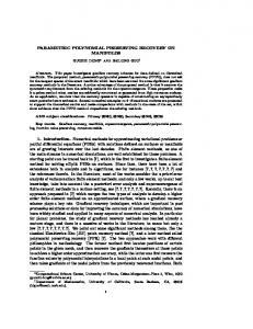
> CellPlot(r, 48); From the plot, we see that the point (a, b) = (1, 6/5) lies in the 48th cell. Let us verify that using the CellLocation command. > CellLocation(r, [a=1,b=6/5]); 48 Therefore, we know that the system has 4 solutions for these parameter values. We can verify this by explicitly computing the solutions, using the command SampleSolutions with a different calling sequence. > SampleSolutions(r, [a=1,b=6/5]); [[x = −0.9901056498, y = −0.2196908022], [x = −0.5472396276, y = −0.9005287899], [x = 0.5472396276, y = −0.9005287899], [x = 0.9901056498, y = −0.2196908022]] We can plot more than one cell at the same time, e.g., the 48th and 54th cells (see Fig. 2) or all cells together (see Fig. 3). The coloring scheme is such that no two adjacent cells have the same color. > CellPlot(r, [48,54]); > CellPlot(r, view=[-10..10,-4..4]); Example 3 The final example is from control theory; we refer the reader to [10] for an introductory text. Suppose we have a feedback control system as in Fig. 4, and that we have identified the transfer function of the plant as P (s) =

s3

+

1 . + 6s + 4

4s2

We want to use a proportional-integral controller, with transfer function C(s) = a + 6

b s


6.

5.

4.

b 3.

2.

1.

0.0

0.2

0.4

0.6

0.8

a

1.0

1.2

1.4

1.6

1.8

Figure 2: The 48th and 54th open cells in Example 2.

4.

3.

b

2.

1.

K

10.

K

0

5.

5.

a

K

1.

K

2.

K

3.

K

4.

Figure 3: All open cells in Example 2.

Figure 4: A feedback control system.

7

10.



to control this plant. The goal is to select the gain parameters a, b > 0 in such a way that the controller-plant system statisfies the Hurwitz stability criterion. This criterion maintains that the transfer function T (s) =

C(s)P (s) , 1 + C(s)P (s)

for the system has no poles with positive real part. After plugging in P (s) and C(s) and simplifying, we obtain T (s) =

as + b . s4 + 4s3 + 6s2 + (a + 4)s + b

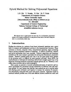
We substitute s = x + iy into the denominator and separate it into real and imaginary parts, Hr (x, y) = x4 − 6x2 y 2 + y 4 + 4x3 − 12xy 2 + 6x2 − 6y 2 + (a + 4)x + b, Hi (x, y) = 4x3 y − 4xy 3 + 12x2 y − 4y 3 + 12xy + (a + 4)y. The Hurwitz criterion is satisfied if Hr (x, y) and Hi (x, y) do not have a common root with x > 0. This leads to the following parametric system:   Hr (x, y) = 0,      Hi (x, y) = 0, x > 0,    a > 0,    b > 0. The following sequence of Maple commands sets up the system and performs the open CAD. > H[r] := x^4-6*x^2*y^2+y^4+4*x^3-12*x*y^2+6*x^2-6*y^2+(a+4)*x+b: > H[i] := 4*x^3*y-4*x*y^3+12*x^2*y-4*y^3+12*x*y+(a+4)*y: > r := CellDecomposition([H[r]=0,H[i]=0,x>0,a>0,b>0], [x,y]): The open CAD contains 15 cells. NumberOfSolutions and CellsWithSolutions are used to find the indices of the admissable cells, namely, the ones where the system has no solutions. > NumberOfSolutions(r); [[1, 0], [2, 2], [3, 0], [4, 0], [5, 2], [6, 2], [7, 0], [8, 0], [9, 2], [10, 2], [11, 2], [12, 0], [13, 2], [14, 2], [15, 2]] > admissible := CellsWithSolutions(r, 0); admissible := [1, 3, 4, 7, 8, 12] Finally, we plot all the admissible cells (see Fig. 5). > CellPlot(r, admissible, color=[red, red, red, red]); From the plot, it looks like the admissible region is the area enclosed by a parabola and the coordinate axes. The equation of the parabola can actually be obtained from the equations of the discriminant variety. > r:-DiscriminantVariety; [[a], [b], [a2 − 16a + 16b − 80], [27a4 + 256a3 − 768a2 b + 768ab2 − 256b3 +768a2 − 1536ab + 768b2 + 768a − 768b + 256]] The last polynomial in the list does not play a role for this question, and we conclude that the admissible region is {(a, b) ∈ R2 : a > 0 and b > 0 and a2 − 16a + 16b − 80 < 0}.

8


9.

8.

7.

6.

5.

b 4.

3.

2.

1.

0 0

5.

10.

a

15.

20.

Figure 5: The admissible region in Example 3.

References [1] G.E. Collins, Quantifier elimination for the elementary theory of real closed fields by cylindrical algebraic decomposition, Lecture Notes in Computer Science, Vol. 33, Springer, 1975, pp.134-183. [2] S. Corvez and F. Rouillier, Using computer algebra tools to classify serial manipulators, Lecture Notes in Artificial Intelligence, Vol. 2930, Springer, 2003, pp.31-43. [3] A. Dolzmann, T. Sturm and V. Weispfenning, Real quantifier elimination in practice, in: B.H. Matzat, G.-M. Greuel and G. Hiss(Ed.), Algorithmic Algebra and Number Theory, Springer, Berlin, 1998, pp.221-247. [4] J.-C. Faugère, A new efficient algorithm for computing Gröbner bases (F4 ), Journal of Pure and Applied Algebra 139 (1999) 61-88. [5] D. Lazard and F. Rouillier, Solving parametric polynomial systems, Journal of Symbolic Computation 42 (2007) 636-667. [6] G. Moroz, Complexity of the resolution of parametric systems of equations and inequations, in: Proc. ISSAC’06, ACM, 2006, pp.246-253. [7] F. Rouillier, Solving zero-dimensional systems through the rational univariate representation, Applicable Algebra in Engineering, Communication and Computing 9 (1999) 433-461. [8] F. Rouillier and P. Zimmermann, Efficient isolation of polynomial real roots, Journal of Computational and Applied Mathematics 162 (2003) 33-50. [9] A. Seidl and T. Sturm, A generic projection operator for partial cylindrical algebraic decomposition, in: Proc. ISSAC’03, ACM, 2003, 240-247. [10] J. Van de Vegte, Feedback Control Systems. 3rd ed., Prentice Hall, 1994.

9