this paper, we propose two new coupling schemes for an implicit coupling of black-box fluid and structure solvers that execute the two solvers in parallel and still ...
V International Conference on Computational Methods for Coupled Problems in Science and Engineering COUPLED PROBLEMS 2013 S. Idelsohn, M. Papadrakakis and B. Schrefler (Eds)
A PARALLEL, BLACK-BOX COUPLING ALGORITHM FOR FLUID-STRUCTURE INTERACTION BENJAMIN UEKERMANN∗ , HANS-JOACHIM BUNGARTZ† , BERNHARD GATZHAMMER† AND MIRIAM MEHL∗ ∗ Institute
for Advanced Study (IAS), Technische Universit¨at M¨ unchen Lichtenbergstraße 2a, 85748 Garching b. M¨ unchen, Germany e-mail: {uekerman,mehl}@in.tum.de, web page: http://www5.in.tum.de † Institut
f¨ ur Informatik, Technische Universit¨at M¨ unchen Boltzmannstraße 3, 85748 Garching b. M¨ unchen, Germany e-mail: {bungartz,gatzhamm}@in.tum.de, web page: http://www5.in.tum.de
Key words: Fluid-Structure Interaction, Strong Coupling, Black-Box Coupling, Partitioned Coupling, High Performance Computing, Scientific Computing Abstract. The simulation of multi-physics scenarios, in particular fluid-structure interaction has gained more and more importance in the last years due to increasing accuracy requirements for a large range of applications from biomedical fields to technical design problems. At the same time, this type of simulation has become feasible due to the increased computing power of modern supercomputers. Note that only the combination of a highly accurate and, thus, highly resolved, discretization with the multi-physics model yields more detailed and more realistic results than a simple single-physics simulation. However, modern computing architectures require a good scalability of simulation methods on massively parallel systems. For fluid-structure interactions, if done in a partitioned way using separate fluid and structure codes, in particular the usually applied staggered scheme executing fluid and structure solver one after the other hinders a good scalability. This is due to the in general largely different computational costs of the two solvers. In this paper, we propose two new coupling schemes for an implicit coupling of black-box fluid and structure solvers that execute the two solvers in parallel and still yield good convergence and stability even for incompressible fluids which is shown by means of numerical results for the flow through a flexible tube. 1
INTRODUCTION
In the last years, modern computational development provided a computational power that allowed to tackle complex multi-physics simulations furthering a new range of industrial and medical applications such as interactions between aircraft wings and the 1
Benjamin Uekermann, Hans-Joachim Bungartz, Bernhard Gatzhammer and Miriam Mehl
surrounding turbulent flow or between blood flow and arterial walls. However, the highly parallel architecture of modern supercomputers, at the same time, poses new challenges that require the development of new numerical algorithms in order to exploit their computational power. The focus of this paper is the development of new numerical algorithms for the example of fluid-structure interactions, where a fluid flow exerts forces on a structure and the structural movement changes the flow field such that we have a bidirectional strong interaction between flow and structural mechanics. 1.1
The modular approach: partitioned black-box coupling
To achieve a high flexibility and modularity of the fluid-structure interaction simulation environment, we focus on a special type of coupling, the so-called partitioned approach. The coupling between different physics in this case takes place at the highest possible level. In fluid-structure interaction (FSI), this is done via boundary conditions at the fluid-structure interface (wet surface). The most common technique is the DirichletNeumann coupling prescribing displacements and velocities as boundary conditions for the flow solver and forces for the structure solver. The counterpart of partitioned methods, monolithic schemes, in contrast, couple at a very low level. They assemble one large system of equations that is solved as a whole and use separate fluid and structure solvers only on a preconditioner level (see e.g. [1]). The disadvantages of partitioned coupling are possible stability issues (cf. e.g. [2]), but this effort is worth taking. By separating the physical regimes, we can reuse existing solver codes and, thus, benefit from the experiences which have been made in each field. Furthermore, non-linear and linear solvers can be better tuned to the particular characteristics each physical system adheres. The clearest advantage, however, of partitioned approaches is the separation of codes. With this approach, solver codes can easily be exchanged permitting the integration of existing codes in a plug-and-play manner. To maximize the flexibility in exchanging codes, we particularly aim at using black-box solvers offering the same technical interface depth as standard commercial solvers usually provide. Thus, the coupling must be formulated independently of the spatial and time discretization of each solver as this is hidden in the black-box. Also Jacobian information is in general not available. Our group developed the coupling environment preCICE 1 , which implements a partitioned black-box coupling, data mapping functionality for non-matching grids, and communication routines. It allows a very flexible and easy exchange of solver codes (cf. [3]). 1.2
Efficient parallelization
Besides numerical coupling methods sketched above, efficient parallelization is the key to highly accurate simulations2 . However, a load balanced parallelization is not trivial 1
http://www5.in.tum.de/wiki/index.php/PreCICE Webpage Note that only a high accuracy in the discretization and solution of multi-physics models accounts for their inherent accuracy. 2
2
Benjamin Uekermann, Hans-Joachim Bungartz, Bernhard Gatzhammer and Miriam Mehl
due to the physical regimes’ cost-asymmetry. Structure calculations typically require far less computational power and, therefore, do not scale well on a high number of processors. Thus, if both physics are solved in a staggered fashion as shown in Fig. 1 (top), i.e., one solver always precedes the other solver, the structure part is a scalability bottleneck. Monolithic schemes can overcome this problem. However, we focus on a black-box partitioned approach, where we develop new numerical algorithms for a parallel, stable, and efficient parallel fluid-structure coupling. For compressible flow, there are explicit coupling schemes known that allow for a high parallel efficiency. This is, e.g., accomplished by a cross-staggered scheme ([4]) or by means of an interface system ([5]) all requiring only one execution of fluid and structure solver per time step resulting in a so-called explicit coupling. Incompressible flow, however, in general needs implicit coupling, i.e., an iterative coupling loop over fluid and structure solution steps during every timestep. This is due to the different nature of the added mass effect in the incompressible case inducing well-known stability issues ([2, 6, 7]). A straightforward generalization of the classical explicit parallel methods in [4] to implicit coupling leads to redundant computations, whereas the methods in [5] require discretization details in the vicinity of the wet surface and, thus, conflict with black-box solvers. Classical implicit black-box approaches follow the staggered scheme. In the simplest form, they use (Aitken-) underrelaxation (see e.g. [8]) to achieve stability. Degroote et al. [9] describe a black-box algorithm that instead solves an interface equation by means of a quasi-Newton approach (IQN), which behaves like an implicit time-integration scheme in an ODE context. The theoretical background of this method was discussed in [10]. Similar methods have been proposed in [11], [12] and [13]. The drawback of all mentioned implicit coupling algorithms is, however, that fluid and structure are still solved in a staggered way causing a bad parallel efficiency. In this paper we present and discuss two implicit coupling algorithms that simulate structure and fluid simultaneously, leading to a high parallel efficiency. We test these methods by means of a simple one-dimensional toy problem, the flow through a flexible tube. The structure of this paper is as follows. In Sect. 2, the two new parallel, implicit coupling algorithms will be introduced. In Sect. 3, we describe the one-dimemensional application example that we use to test our new methods, covering the analytical description as well as the discretization technique. Numerical results for this example are shown in Sect. 4. We close the paper with conclusions and an outlook in Sect. 5. 2
TWO PARALLEL IMPLICIT COUPLING ALGORITHMS
In the following, we introduce our new parallel implicit coupling algorithms in two steps. First, we revisit the quasi-Newton least square (QNLS) method described in [10]. Then, we use this method to solve different abstract fixed point equations leading us to the new coupling algorithms. To close the section, we discuss different convergence criteria.
3
Benjamin Uekermann, Hans-Joachim Bungartz, Bernhard Gatzhammer and Miriam Mehl
2.1
Quasi-Newton least squares method
We start from a non-linear fixed point equation, find x ∈ D ⊂ Rn , such that H(x) = x ,
(1)
where H : D → Rn is sufficiently smooth and has a unique fixed point x∗ ∈ D. The Jacobian of the residual R(x) = H(x) − x at x∗ , i.e. R0 (x) = H 0 (x∗ ) − I, is assumed to be non-singular. We approximate the solution x∗ in an iterative quasi-Newton manner, i.e., we solve an approximation of the linearized equation � � � (2) R0 xk x − xk = −R xk in every iteration. As we want to be able to use black-box � solvers in our fluid-structure simulations, we have no access to the Jacobian R0 xk . However, we can use in- and output data of the functions H and R to approximate the solution of (2). We assume that we already have a sequence x0 , . . . , xk and the corresponding output values x˜0 = H(x0 ), . . . , x˜k = H(xk ). We further assume that the input vectors x0 , . . . , xk are linearly independent. With this, we can construct the two matrices k V k = [∆R0k , . . . , ∆Rk−1 ] k k k W = [∆x0 , . . . , ∆xk−1 ]
with with
∆Rik = R(xk ) − R(xi ), i = 0 . . . k − 1 , and ∆xki = xk − xi , i = 0 . . . k − 1 .
(3) (4)
To set xk+1 , we construct ∆xk := xk+1 − xk in the column space of Wk : ∆xk = Wk α such that (2) is solved as accurately as possible. For this purpose, we solve a least squares
� problem α = argminβ∈Rk V k β + R xk 2 , where k·k denotes the Euklidian norm in Rn . To solve this least squares problem, we compute the decomposition V k = Qk U K of V k into an orthogonal n × n matrix Qk and an upper triangular matrix U k ∈ Rn×k and compute α from the quadratic k × k system � �T � ˜ k R xk , U˜ k α = − Q (5) ˜ k contains the first k columns of Qk . where U˜ k denotes the first k rows of U k and Q With α, we can approximate the solution of (2) as xk+1 − xk := W k α
(6)
since this gives −R x
k
�
k
≈V α=
k−1 X i=0
k−1
αi ∆Rik
� � � �X . = R 0 xk αi ∆xki = R0 xk W k α = R0 xk xk+1 − xk . i=0
As the quasi-Newton method requires at least one column in V k and W k , we have to use simple underrelaxation for the first iteration: x1 = x0 + 0.1 · R(x0 ). However, with this 4
Benjamin Uekermann, Hans-Joachim Bungartz, Bernhard Gatzhammer and Miriam Mehl
approach, we get a new iterate xk+1 that is a linear combination of x0 , . . . , xk and, as a consequence, we get quasi-Newton iterates in the two-dimensional space span {x0 , x1 }3 . For this reason, we modify the method a little: We replace W k in (4) by xkk−1 ] with ∆˜ xki = x˜k − x˜i , i = 0 . . . k − 1 . W k = [∆˜ xk0 , . . . , ∆˜ This corresponds to approximating the solution of � � � � �0 R ◦ H −1 x˜k xk+1 − x˜k = −R ◦ H −1 x˜k = −R xk
(7)
(8)
instead of (2). This a fixed point iteration step � results in a methods that performs first k k k k x → x˜ = H x and afterwards a quasi-Newton step x˜ → xk+1 approximately solving (8) with (5) and (6) with x˜k instead of xk and R ◦ H −1 instead of R. See Algorithm 1 for the complete algorithm. Algorithm 1 Quasi-Newton least squares method in pseudocode initial value x0 x ˜0 = H(x0 ) and R0 = x ˜ 0 − x0 1 0 0 x = x + 0.1 · R for k = 1 . . . do x ˜k = H(xk ) and Rk = x ˜ k − xk k ] with ∆Rk = Ri − Rk V k = [∆R0k , . . . , ∆Rk−1 i k k xki = x ˜i − x ˜k xk−1 ] with ∆˜ Wk = [∆˜ x0 , . . . , ∆˜ decompose V k = Qk U k T solve the first k lines of U k α = −Qk Rk ∆˜ x = Wα xk+1 = x ˜k + ∆˜ xk end for
In a transient fluid-structure context, i.e., if we perform quasi-Newton iterations in every timestep, the initial value x0 for the current timestep can be extrapolated. Furthermore, the reuse of iteration values x˜i and R(xi ) from previous timesteps in order to construct V and W accelerates the convergences (compare [9] and Sect. 4). 2.2
Coupling variants induced by fixed point equations
With the general formulation of the QNLS method in Sect. 2.1, different coupling algorithms can be constructed by formulating the corresponding fixed point equations. For this sake, we use an abstract notation for the fluid and structure solver action on the wet surface between fluid and structure. This notation is typically used for the description of partitioned approaches (see e.g. [14]) and can be stated independently of the solver 3
At the same time, also the columns of V k are ’almost parallel’, i.e., the QU -decomposition becomes ill-conditioned.
5
Benjamin Uekermann, Hans-Joachim Bungartz, Bernhard Gatzhammer and Miriam Mehl
details. Let F : d 7→ f be the mapping of interface displacements to interface forces induced by the fluid solver and S : f 7→ d the mapping of forces to displacements induced by the structure solver, i.e., force and displacements at the wet surface are denoted by f and d, respectively. Figure 1 shows schematic views of different coupling algorithms together with the corresponding fixed point equations. d
f
F
S
d
d
F
d
F
f
IQN
d
F
f
d
S −1
f
d
S −1
d
F
f
d
f
S
d
f
f
d
S
IQN
d
d
F
f
f
d
S −1
f
F
f
d
F
f
S
d
f
S
d
PIQN
(S −1 − F )(d) + d = d
PIQN
VIQN
(S ◦ F )(d) = d
VIQN
�
0 S F 0
�� � � � d d = f f
(9) (10)
(11)
Figure 1: Coupling variants and their corresponding fixed point equations. (9) yields the well-known staggered interface quasi-Newton (IQN) approach (cf. [9]). (10) and (11) define our new algorithms, which we call parallel interface quasi-Newton (PIQN) and vectorial interface quasi-Newton (VIQN).
The fixed point equation (9) yields the classical interface quasi-Newton (IQN) algorithm described in [9]. This algorithm evaluates F and S in serial causing a bad parallel efficiency as described in Sect. 1. A good parallel performance can only be achieved if F and S can be evaluated in parallel as in (10) and (11). The method in (11) (which we call vectorial interface quasi-Newton or VIQN) is closely related to the parallel explicit method in [4]. Both solvers have the usual input (displacements and velocities for the fluid solver and forces for the structure solver). After one iteration of both solvers, the output boundary values are exchanged and the next iteration is started. Doing this without the quasi-Newton least squares step after each iteration would lead to two disconnected instances of the usual staggered iterations. However, the quasi-Newton steps introdce a connection. Section 4 shows that this connection is indeed strong enough to make one iteration of VIQN comparable to one iteration of IQN. The second parallel coupling scheme (10) (called parallel interface quasi-Newton or PIQN) uses the inverse interface structure operator S −1 : d 7→ f . For the structure solver, this inversion yields no higher costs, standard commercial solvers allow for this inverse formulation. Thus, both solvers compute forces at the interface as an output. If the iterations are converged, these two forces have to be the same. Thus, we actually solve the equation (S −1 − F )(d) = 0 to determine the new interface displacements used as an input for the next iteration. 2.3
Convergence criterion
The choice of a particular convergence criterion to compare the different algorithms presented in the last subsection is a delicate issue. The QNLS algorithm as itself induces 6
Benjamin Uekermann, Hans-Joachim Bungartz, Bernhard Gatzhammer and Miriam Mehl
the relative criterion k˜ xk − xk k < tol · kxk k .
(12)
For the IQN algorithm, this criterion checks only for the convergence of the displacement values where for VIQN displacement as well as force values are checked. Furthermore, for VIQN, an equal weight of both physical values is not guaranteed. Therefore, we prefer a physically motivated approach to compare the different coupling algorithms with a uniform convergence criterion: kd˜k − dk k < tol · kdk k and kf˜k − f k k < tol · kf k k . 3
(13)
PROBLEM DESCRIPTION
In this section, we shortly describe the flow through a flexible tube which we use for testing our new coupling algorithms. The model and the description follow [14]. 3.1
Analytical description
The fluid flow in our example is incompressible and inviscid, and no gravity is assumed. Averaging over the tube in radial directions yields a one-dimensional model as displayed in Fig. 2. The conservation of momentum and mass read ∂t (au) + ∂x (au2 ) + a∂x p ∂t a + ∂x (au)
= 0, = 0,
(14) (15)
where u is the flow velocity in axial direction, p the kinematic pressure, and a the cross section area of the tube. We impose a time-varying inlet velocity and a non-reflecting outlet boundary condition: t 1 u0 sin2 (π ) and ∂t u = ∂t p , (16) 100 T c p where c2 := dap a = c2mk − p2 is the wave speed, cmk = Eh/2ρr0 the Moens-Korteweg wave speed and E Young’s modulus. The elastic wall is described by a Hookean constitutive law. Since the inertia of the tube wall is neglected, the wall contains no mass. This fact in combination with the incompressibility of the fluid constitutes a severe test for coupling algorithms, because it tightens the instabilities induced by the added mass effect, which depends on the density relation between fluid and structure. The inviscid fluid exerts only stress in circumferential direction on the structure leading to a purely radial motion of the tube wall. As a consequence, the cross section area becomes an explicit function of the pressure: � �2 p0 − 2c2mk a = a(p) = a0 (17) p − 2c2mk uin = u0 −
7
Benjamin Uekermann, Hans-Joachim Bungartz, Bernhard Gatzhammer and Miriam Mehl
x
r
p
p
r
σϕϕ
h σϕϕ
L
Figure 2: Schematic drawing of the deformed tube with flow in x-direction, inner radius r = r(x), length L, and wall thickness h. The fluid pressure p(x) acting on the inner tube walls is causing scalar circumferential stresses σϕϕ (x) in the tube walls which lead to a deformation in radial direction. The test scenario is based on [14].
with a0 and p0 being reference values. For details of the model, refer to [14]. Thus, for this scenario, the general coupling variables force f and displacement d are substituted by the pressure p and the cross section area a. We simulate the scenario over a time interval [0; T ], a full period of the inlet velocity. 3.2
Discretization
The tube of length L is subdivided into NS equidistant cells of length ∆x = L/NS with values ui , pi and ai assigned to the cell centers4 . Equation (14) and (15) are discretized with finite volumes using central discretization schemes in combination with a first-order upwind scheme for the convective term in the momentum equation. The central discretization scheme of the pressure is stabilized by a pressure stabilization with coefficient a0 . For time discretization of the fluid equations, we use a backward Euler α = u0 +∆x/∆t scheme and subdivide [0, T ] into NT equidistant slots of length ∆t. The discretized system yields for all spatial segments i = 1, . . . , N − 1 � h i(n+1) ∆x � (n+1) (n+1) (n) (n) − ui ai + ui ui+ 1 ai+ 1 − ui−1 ui− 1 ai− 1 ai ui 2 2 2 2 ∆t h i(n+1) 1 + ai+ 1 (pi+1 − pi ) + ai− 1 (pi − pi−1 ) = 0 , (18) 2 2 2 � h i(n+1) h i(n+1) ∆x � (n+1) (n) ai − ai + ui+ 1 ai+ 1 − ui− 1 ai− 1 − α pi−1 − 2pi + pi+1 = 0 . (19) 2 2 2 2 ∆t The subscript i ± 1/2 indicates the values calculated at the cell interfaces, e.g., ui−1/2 = 0.5 · (ui−1 + ui ). The superscripts (n) and (n + 1) refer to time t(n) = n · ∆t and t(n+1) = (n + 1) · ∆t, respectively. The pressure value at the inlet and the velocity value at the outlet are linearly extrapolated (pin = 2p1 − p2 and uout = 2uN − uN −1 ), whereas the pressure-outlet condition is discretized as !2 r n n p uout − uout pout = 2 c2mk − c2mk − out − . (20) 2 4 4
This means, we use the same grid for the fluid and the structure solver.
8
Benjamin Uekermann, Hans-Joachim Bungartz, Bernhard Gatzhammer and Miriam Mehl
The velocity values ui , the pressure values pi , and the cross section area values ai are initially set to their reference values u0 , p0 , and a0 . To achieve comparablepresults, we follow the idea of [14] and define the dimensionless structural stiffness κ = ( Eh/2ρr0 − p0 /2)/u0 and the dimensionless timestep size τ = u0 ∆t/L as physical parameters of our scenario. We fix NS = 100 and NT = 100. The stability analyses in [14], as well as in [2] and [7] show that achieving stability for the FSI coupling gets more challenging with decreasing structural stiffness κ or decreasing timestep size τ . 4
NUMERICAL RESULTS
In this section, we discuss the numerical results obtained for our new parallel coupling algorithms introduced in Sect. 2 if applied to the problem from Sect. 3. Figure 3 shows results for the cross section area for different timesteps. All results presented in this paper yield the same values for u, p, and a as a quasi-monolithic approach (for details see [14]) up to an l2 -error of 10−7 . 10
1.001
IQN(5) VIQN(5) PIQN(5)
1
Number of iterations k
Cross section a/a0
t/T=0.2 1.001 t/T=0.4 1
1.001 t/T=0.6
1
8 6 4 2
1.001 t/T=0.8 1 0
0.2
0.4 0.6 Spatial coordinate x/L
0.8
0
1
Figure 3: Cross section area values a/a0 for different timesteps during one simulation. The dimensionless timestep size for this run is τ = 0.01 and the dimensionless structural stiffness is κ = 10. All coupling algorithms yield the same values a up to an error of 10−7 .
2
4
6
8 10 Timestep
12
14
Figure 4: Coupling iteration numbers for the first 15 timesteps. IQN shows less iteration numbers than VIQN in the beginning, but is surpassed by VIQN after 3 timesteps. The dimensionless timestep size for this run is τ = 0.01 and the dimensionless structural stiffness is κ = 100.
For the performance discussion of the different algorithms, we assume that all interface calculations are negligible in terms of computational costs compared to the fluid and the structure solver calculations. This assumption holds for real applications, where, in contrast to the toy problem used in this paper, the fluid and the structure domain have a higher dimensionality than the wet surface. Results in [9] confirmed this assumption. As a consequence, the number of solver calls, hence the number of coupling iterations, is a sufficient estimator of the computational costs. We use the convergence criterion discussed in Sect. 2.3 in an l2 -sense with tol = 10−7 . We test the two new algorithms PIQN and VIQN introduced in Sect. 2 against the IQN algorithm of [9] for different values of the dimensionless timestep size τ and the dimensionless structural stiffness κ. By IQN(5), e.g., we denote the IQN algorithm with 9
Benjamin Uekermann, Hans-Joachim Bungartz, Bernhard Gatzhammer and Miriam Mehl
the reuse of the values from the last 5 timesteps. Table 4 shows the average numbers of resulting coupling iterations. The optimal number of reused timesteps depends on the Table 1: Average coupling iteration numbers for the different fixed point equations and different solver parameters τ and κ. For each method, the average iteration numbers with no reuse of vectors are shown in the top half of the table. The lower half shows the results using reuse of previous vectors. Here, only the best configuration are presented, which are the reuse of 5 previous steps for IQN, respectively 8 and 5 for VIQN and PIQN.
IQN
VIQN
PIQN
τ \κ 1000 100 10 0.1 3.96 4.07 5.59 0.01 3.97 5.01 9.19 0.001 5.00 9.09 28.4
τ \κ 1000 100 10 0.1 4.09 4.22 6.68 0.01 4.08 6.05 13.5 0.001 6.00 12.4 40.9
τ \κ 1000 100 10 0.1 3.97 4.35 6.75 0.01 4.06 5.39 13.7 0.001 5.28 10.2 26.5
IQN(5)
VIQN(8)
PIQN(5)
τ \κ 1000 100 10 0.1 2.99 3.04 3.25 0.01 3.02 3.09 3.58 0.001 3.07 3.28 6.83
τ \κ 1000 100 10 0.1 2.08 2.07 2.36 0.01 2.08 2.12 3.15 0.001 2.11 2.66 8.53
τ \κ 1000 100 10 0.1 3.01 3.09 3.55 0.01 3.05 3.20 4.58 0.001 3.08 3.75 8.63
parameters, but is in general higher for VIQN than for IQN and PIQN. For our test scenario, the reuse of iterations from 8 previous timesteps results, for most parameter settings, in the smallest number of iterations for VIQN, whereas for IQN and PIQN, the reuse of 5 timesteps was optimal. The number of iterations increases, in general, with decreasing dimensionless timestep size τ , and decreasing dimensionless structural stiffness κ. PIQN shows competitive results, but slightly worse than IQN and VIQN. VIQN needs, in most cases, even less coupling iterations than IQN. The time evolution of the iteration numbers clarifies this fact. Figure 4 shows the iteration numbers for the first 15 timesteps of each method for one exemplary parameter setting. In the first timesteps, IQN needs less iterations than VIQN, but this changes quickly after 3 timesteps. In principle, the fixedpoint equation behind IQN is more suited for the coupling, since the force variables f and the displacement variables d are more interconnected compared to the VIQN fixed-point equation. VIQN, however, benefits more from the reuse of previous timesteps because force values can also be reused instead of just displacements. A better understanding of the difference between VIQN and IQN can be obtained by looking at the absolute errors (compare Fig. 5). VIQN shows a worse convergence than IQN while VIQN(5) outperforms IQN(5). Moreover, VIQN shows smaller absolute errors already in the first iterations due to the extrapolation of the pressure values - for IQN only the displacements are extrapolated. Furthermore, a small oscillation of the VIQN residuals without the reuse of previous timesteps can be observed, due to the underrelaxation step in the first iteration yielding a shifted influence on the pressure p and cross section area 10
Benjamin Uekermann, Hans-Joachim Bungartz, Bernhard Gatzhammer and Miriam Mehl
values a. As the reuse of previous timesteps supersedes the starting underrelaxation step, this feature disappears for VIQN(n) with n > 0. 0
0
10
Absolut Error
Absolut Error
10
−5
10
−10
10
IQN area IQN pressure VIQN area VIQN pressure PIQN area PIQN pressure
0
IQN(5) area IQN(5) pressure VIQN(5) area VIQN(5) pressure PIQN(5) area PIQN(5) pressure
−5
10
−10
10
5
10
0
15
5
10
Iteration k
Iteration k
Figure 5: Absolute errors kak − a20 k∞ , kpk − p20 k∞ of different coupling algorithms. On the left side, the simple coupling algorithms are shown, while on the right side, the values from the previous 5 timesteps are reused. The dimensionless timestep size for this run is τ = 0.001 and the dimensionless structural stiffness is κ = 10. We used a stricter convergence criterion for this simulations to show a longer development of the errors. All residuals are plotted exemplary for timestep 30.
5
CONCLUSIONS AND OUTLOOK
We have presented two new algorithms exploiting the potential of interface quasiNewton methods for a parallel instead of a staggered coupling in fluid-structure interaction simulations. These methods are important steps towards scalable massively parallel fluid-structure simulations. The numerical results for an incompressible flow through an massless flexible tube showed the large potential of our methods. In particular, the VIQN method that has the additional advantage of not changing the boundary conditions used for fluid and structure in common staggered Dirichlet-Neumann methods, proved to be very efficient. The performance of the PIQN method is slightly worse. It turned out that for parallel coupling the reuse of information from previous timesteps is of crucial importance. The choice of an optimal number of steps to reuse is, however, still an open issue and subject of future work as well as the implementation of the method for more general two- and three-dimensional examples and supercomputing architectures. Acknowledgement The financial support of the Institute for Advanced Study (IAS) of the Technische Universit¨ at M¨ unchen is thankfully acknowledged.
REFERENCES [1] Bazilevs, Y., Takizawa, K. and Tezduyar, T. E. Computational Fluid-Structure Interaction - Methods and Applications. John Wiley and Sons, Vol. I., (2013). [2] Causin, P., Gerbeau, J. F. and Nobile, F. Added-mass effect in the design of partitioned algorithms for fluid-structure problems. Comput. Methods Appl. Mech. Eng. (2005) 194:4506–4527.
11
Benjamin Uekermann, Hans-Joachim Bungartz, Bernhard Gatzhammer and Miriam Mehl
[3] Bungartz, H.-J., Benk, J., Gatzhammer, B., Mehl, M. and Neckel, T.: Partitioned Simulation of Fluid-Structure Interaction on Cartesian Grids. In Bungartz, H.-J., Mehl, M., Sch¨afer, M., editors. Fluid-Structure Interaction – Modelling, Simulation, Optimisation, Part II. Lecture notes in CSE. Berlin, Springer (2010) 73:255–284. [4] Farhat, C. and Lesoinne, M. Two efficient staggered algorithms for the serial and parallel solution of three-dimensional nonlinear transient aeroelastic problems. Comput. Method. Appl. M. (2000) 182:499–515. [5] Ross, M.R., Felippa, C.A., Park, K.C. and Sprague, M.A. Treatment of acoustic fluid-structure interaction by localized Lagrange multipliers: Formulation. Comput. Methods Appl. Mech. Eng. (2008) 197:305–3079. [6] F¨orster, Ch., Wall, W. A. and Ramm, E. Artificial Added Mass Instabilities in Sequential Staggered Coupling of Nonlinear Structures and Incompressible Viscous Flows. Comp. Meth. Appl. Mech. Eng. (2007) 196:1278–1293. [7] Van Brummelen, E. H. Added Mass Effects of Compressible and Incompressible Flows in Fluid-Structure Interaction. J. Appl. Mech. (2009) 76. [8] K¨ uttler, U. and Wall, W. Fixed-point fluid-structure interaction solvers with dynamic relaxation. Comput. Mech. (2008) 43:61–72. [9] Degroote, J., Bathe, K.-J. and Vierendeels, J. Performance of a new partitioned procedure versus a monolithic procedure in fluid-structure interaction Comput. Struct. (2009) 87:793–801. [10] Haelterman, R., Degroote, J., Van Heule, D. and Vierendeels, J. The Quasi-Newton Least Squares Method: A New and Fast Secant Method Analyzed for Linear Systems. SIAM J. Numer. Anal. (2009) 47:2347–2368. [11] Vierendeels, J. Implicit coupling of partitioned fluid-structure interaction solvers using reduced-order models. In: Bungartz, H.-J., Sch¨afer, M., editors. Fluid-Structure Interaction – Modelling Simulation, Optimisation. Lecture notes in CSE. Berlin, Springer (2006) 53:1–18. [12] Michler, C., van Brummelen, E. and de Borst, R. An interface Newton-Krylov solver for fluid-structure interaction. Int. J. Numer. Methods Fluids (2005) 47:1189–1195. [13] Gerbeau, J. F., Vidrascu, M. A quasi-Newton algorithm based on a reduced model for fluid-structure interaction problems in blood flows. Math. Model. Numer. Anal. (2003) 37:631–648. [14] Degroote, J., Bruggeman, P., Haelterman, R. and Vierendeels, J. Stability of a coupling technique for partitioned solvers in FSI applications. Comput. Struct. (2008) 86:2224–2234.
12