We show that the method performs accurately and at interactive rates, even for large feature areas ... Figure 1: a) âLucyâ model (200K) colorized with mean cur-.
A Parametric Space Approach to the Computation of Multi-Scale Geometric Features Anthousis Andreadis
Georgios Papaioannou
Pavlos Mavridis
Department of Informatics, Athens University of Economics and Busines, Athens, Greece {anthousis, gepap, pmavridis}@aueb.gr
Keywords:
Geometric features, Parametric space, Mesh geometry
Abstract:
In this paper we present a novel generic method for the fast and accurate computation of geometric features at multiple scales. The presented method works on arbitrarily complex models and operates in the parametric space. The majority of the existing methods compute local features directly on the geometric representation of the model. Our approach decouples the computational complexity from the underlying geometry and in contrast to other parametric space methods, it is not restricted to a specific feature or parameterization of the surface. We show that the method performs accurately and at interactive rates, even for large feature areas of support, rendering the method suitable for animated shapes.
1
INTRODUCTION
Geometric features, like curvature and surface roughness, are central to demanding computations in a wide range of applications, including object retrieval and registration, texture synthesis, stylized rendering and many more. The computation of these fundamental metrics is usually performed by CPU algorithms that operate on a discrete polygonal representation of a continuous surface. These metrics can be precomputed for static meshes, but their fast computation even for moderately large or dynamic meshes, is challenging. In this paper we focus on the general class of metrics with finite local support, whose computation depends on the local neighborhood of an arbitrary point p on the object’s surface. Robustness in the presence of noise is achieved through multi-scale computation of the features (Yang et al., 2006). To this end, a data structure that encodes the adjacency information is required, in order to efficiently locate the neighboring points on a surface. This is especially true for algorithms that operate on meshes. The computational complexity of such an object-space approach is directly proportional to the geometric density and quadratic with respect to the extent (i.e. radius) of the local feature support. Despite the fact that computing the metric for independent surface points is an inherently parallel task, the use of complex data structures for storing the adjacency information prevents a trivial and efficient mapping of these computations to
Figure 1: a) ”Lucy” model (200K) colorized with mean curvature, computed in 49ms, b) geometry (position) buffer (normalized for visualization), c) surface normal buffer, d) polygon chart identifiers (colorized for clarity) along with the adjacent chart identifiers on border pixels, e) mean curvature in parametric space (colorized for visualization).
massively parallel stream processors, like commodity GPUs, at an arbitrary neighborhood scale. For these reasons, real-time computation is often limited to meshes with relatively low geometric complexity and 1-ring vertex neighborhoods (Griffin et al., 2011). Our approach for local feature computation shifts all calculations from object-space to parametric
space, by transferring all the geometric data of the object to a two-dimensional layout, along with extra adjacency information that allows us to reconstruct the object-space local neighborhood of a given point on the fly. While this choice is similar to Geometry Images (Gu et al., 2002), we do not restrict our method to a specific parameterization method, but rather develop a scheme that can handle any underlying parameterization, including multi-chart layouts. The benefits of parametric-space feature calculations are twofold: First, sampling the geometry at arbitrarily large areas of support is much more efficient in parametric space, since the samples can be directly indexed in contrast to a geometry-based estimation, where the traversal of a surface patch is performed via the connectivity information of the vertices. Second, the parametric space computations are directly mapped to the GPU/many-core computing paradigm in a very efficient manner, rendering the approach suitable for real time calculations over deformable or animated objects.
2
RELATED WORK
Most methods in the bibliography concentrate on the computation of a specific geometric feature, and do not generalize their framework to encompass more features. Since our method is more generic, for our overview, we focus on the way each method samples the geometric information of the object, instead of the particular feature computation. Existing methods can be classified to those that sample the geometry in object-space, screen space, a volumetric representation and parametric space. In the remainder of this section we will review the main representatives for each category. Object-space methods operate directly on the geometry of the mesh. (Taubin, 1995) and (Meyer et al., 2003) generalize the differential-geometrybased definition of curvatures to discrete meshes but their computations are limited to 1-ring neighborhoods which renders them sensitive to noise. Similarly (Rusinkiewicz, 2004) estimate the curvature over meshes using essentially a 2-ring neighborhood. For efficient arbitrary neighborhoods (support regions), object space methods require a data structure that encodes the adjacency information between the triangles of the mesh, such as the half-edge (Campagna et al., 1998) or a kd-tree data structure. However, as discussed in the introduction, a mapping of this data structure to the GPU is neither trivial nor optimal. Most feature computation methods belongs to this category and thus operate on the CPU. GPU-
based methods, have been proposed for the computation of specific features, like curvature (Griffin et al., 2011), but these methods do not generalize to the sampling of arbitrary neighborhoods. Screen space methods sample the geometric information of a mesh from a 2D pixel buffer, where each pixel encodes the projected surface position of the mesh from a specific point of view. In this case, adjacency information is implied by the pixel grid, therefore sampling is trivial and can be efficiently mapped to GPUs. This efficiency in sampling is also the main motivation behind our method. The main disadvantage of screen-space methods is that computations are limited to the surface points visible from a particular view, resulting in inaccuracies near occluded points and at the screen-space silhouettes of the object. Such screen-space methods have been proposed for curvature estimation in real-time stylized rendering (Mellado et al., 2013), (Kim et al., 2008). Our method retains most of the sampling efficiency of the screenspace methods, but avoids the view-dependence of the results by moving all the computation to the parametric space. Volumetric data and algorithms can be also employed for feature computations. In this case, the input mesh is initially converted to a volumetric representation, such as a level set, and then geometric features are computed by sampling this representation, instead of the original mesh. Finally, the results of these calculations are mapped to the original mesh. The advantage of this approach is that the computational complexity does not depend on the underlying geometry but rather on the new volumetric representation, where sampling a local neighborhood around a surface point is often more efficient than sampling the same neighborhood on the original geometry. Features, like curvature, can be quickly approximated using the gradient field of the object, as described in the OpenVDB (Museth, 2013) or by using convolutions, which can be accelerated using FFT as shown in (Pottmann et al., 2007). The disadvantage of this approach is that an efficient voxelization method is required, additional memory is consumed for the storage of the volumetric format and most importantly, the computations are based on a volumetric discretization, which is a more rough representation of the original surface than the triangular mesh. Furthermore, certain features when computed on volumetric data, are incompatible with the results of the respective surface-based measurements, especially for non-manifold surfaces. Parametric space. Finally, specific methods have been proposed for parametric space as well. Methods in this category rely on a the unwrapped surface of the model on a 2D plane. Using this rep-
resentation, computational complexity is decoupled from the underlying geometry and additionally, several image analysis techniques can be applied intuitively to 3D data. To our knowledge, so far there has been no practical and generic approach that would allow both geometric and image space features to be computed efficiently, as existing methods focus on applying image space techniques only. (Novatnack and Nishino, 2007) propose a method for corner and edge detection that requires a user-driven single chart parametrization. Furthermore, to handle points lying near the perimeter of charts, the authors construct complementary parameterizations, for which boundary regions are then mapped to internal chart locations. (Hua et al., 2008) describe another method that locates extrema using a scale space representation. Their method relies on a specialized conformal mapping and expects pre-computed per-vertex values of mean-curvature and geodesic distance. In contrast, our method does not rely on a specific parameterization approach, nor does it require any pre-computed features.
3
METHODOLOGY
Our method operates on fully parameterized geometry but does not rely on a specific method for this task. Initially, we perform a pre-processing step in order to locate the surface edges of the polygonal representation, which are mapped to discontinuous regions in parametric space. This is usually part of the model loading process. In real-time, we create the parametric-space representation of the geometry, augmented by the adjacency information and perform the feature computation of discrete locations in parametric space, i.e. on a texture buffer. During this step, we utilize the information stored in our geometry and adjacency buffers in order to index arbitrary surface samples in the neighborhood of a point p, regardless of its parametric mapping. The measured metrics can be then queried per vertex, using standard texture look-up operations, or used directly in image space, e.g. to extract salient features and local image-space descriptors. In the rest of this section we will present in detail each one of the above steps.
3.1
Surface Parameterization
Surface parameterization as (Floater and Hormann, 2005) explain, can be viewed as a one-to-one mapping from a suitable domain to a surface. Our method expects fully parameterized geometry in a normalized 2D domain. This procedure is also known as (bijec-
Figure 2: The ”bunny” model with two parameterizations, resulting in different set of charts.
tive) uv-mapping and the resulting surface patches are referred to as charts or uv-islands (see Figure 1(d), and 2). The area of surface parameterization has been extensively researched in the past years, (Floater and Hormann, 2005), (Sheffer et al., 2006) and the minimization of stretch distortion has been the goal of several works, such as that of (Sander et al., 2001), (Yoshizawa et al., 2004) and (Zhou et al., 2004). Therefore, we do not address this part in our work, but rather rely on existing methods and solutions.
3.2
Pre-Processing Operations
In any local feature estimation technique, we need to calculate an operator F(p, S(p)) at a point p, given a neighborhood x ∈ S(p), x satisfying a set of criteria, such as a maximum Euclidean or geodesic distance from p, or the n-ring adjacency of x to p (max. n vertex graph distance). These relations in geometric space are easily represented using data structures with topology. For a review of the existing geometric data representations, see the work of (De Floriani and Hui, 2005). On the other hand, when operating in 2D parametric space, the connectivity information is implied by the adjacency of neighboring pixels. However, this is not true on the borders of charts, where adjacent geometry is mapped to discontinuous locations in parametric space (see example in Figure 3). In this case, additional information should be stored at the border pixels to keep track of the hops to geometricallyadjacent pixels in different charts. In order to appropriately annotate the chart pixels, mesh vertices located at the borders of charts must be first identified and the link to the geometrically adjacent vertices on different charts has to be stored on the affected vertices. Details regarding the information stored can be found in Section 3.3. The complexity of this step is equivalent to the pre-processing stage of all object-space approaches for the adjacency information generation and even for large models, it only takes a few seconds to complete. This stage needs to be performed only once, as the adjacency information for topologically unchanging geometry can be stored in the 3D model file itself.
3.3
Generation of the Data Buffers
The computation of geometric features requires a set of attributes per sampled surface location, such as the coordinates of p in the object’s local space and the respective normal vector n. These data must be transferred to the parametric space and stored in appropriate buffers, i.e. a set of textures that correspond to the normalized parametric space of the unwrapped geometry. The buffers also store the identifier of the polygon chart that p belongs to. The object-space position of surface points is stored in a geometry buffer P(u, v), the normal vectors are placed in a normal buffer N(u, v), whereas the chart identifiers are registered in an ID channel in the geometry buffer (ID(u, v)). Another set of textures, comprising the adjacency buffer, equal in size to the geometry buffer, store the identifier of the adjacent chart, the local metric distortion of the parameterization (see below), the corresponding (u, v) coordinates on the adjacent chart, as well as the relative scale and rotation between the two charts. An example of the data channels for the position, normal and current and adjacent chart identifiers is shown in Figure 1. The buffer generation process is performed in two steps. First, the geometric information is efficiently generated in the GPU by rasterizing the object triangles using orthographic projection, where the normalized texture coordinates (u, v, 1) are used as the vertex coordinates of the mesh. The chart ID is passed as a vertex attribute and copied for all points inside the triangles of a chart. Similarly to (Sander et al., 2003) we also rasterize each chart’s boundary edges in order to avoid the generation of disconnected regions. In the second step, we compute the local metric distortion factors that will be used for the anisotropic adjustment of scale and sampling direction in various calculations. In order to do so we use the Jacobian JP = (Pu , Pv ), where Pu and Pv the partial derivatives of the surface. The left-singular vectors of JP are used in order to get the θe angular distortion of the anisotropic ellipse while the singular values of JP σu , σv are the stretch factors in the u and v direction. Due to the fact that the singular value decomposition is a tedious task, we use the equivalent eigen decomposition of the 2x2 first fundamental form matrix: � � E F T , (1) JP JP = F G where E = (∂P(u, v)/∂u)2 , G = (∂P(u, v)/∂v)2 and F = (∂P(u, v)/∂u) · (∂P(u, v)/∂v). For more information see (Hormann et al., 2008). Additionally, in this second pass we also store the rest of the adjacency data. These attributes are calculated when setting up the triangle connectivity and are simply copies to the
Figure 3: Indexing a sample inside the neighborhood of a point. Sample t does not lie inside the chart of s. Locate the boundary point b, read adjacency buffers and relocate sample to adjacent chart.
adjacency buffers for the chart border pixels. While for static objects the buffer generation step could be performed only once, we focus on a method suitable for deformable/animated objects, and treat it as a perframe event. Therefore, the reported timings in the remaining text include the data buffer generation overhead.
3.4
Sampling the Neighborhood of a Point
In order to be able to perform the calculation of a feature F(p, S(p)) in parametric space, we need to establish a procedure for drawing individual samples from the neighborhood S(p) of p. Our approach estimates F(p, S(p)) in image space and therefore, for every pixel (i, j) with a corresponding parameter pair s = (u, v), p(u, v) is first retrieved from the geometry buffer: p = P(u, v). Then, assuming a maximum radius of support rmax for the local feature estimator in object-space units, a sample t = (u′ , v′ ) is generated in a region A(s) in parametric space so that x = P(t) satisfies the neighborhood criterion. A(s) is calculated as an ellipse of radii (1/σu (s), 1/σv (s)) · rmax in the parametric domain (upper distance bound) rotated by θe , in order to account for local angular distortion and scale, and x is acquired with rejection sampling according to the selected neighborhood criterion (Figure 3). The exact pattern or random distribution with which the samples are generated is specific to the feature estimator and the generic sampling approach presented here is agnostic to it. Also, since we perform a random sampling of the neigborhood of s, no assumption is made about the chart’s convexity. Since the ellipse A(s) may extend beyond the boundary of the chart containing p (Figure 3), a more elaborate mechanism is required to handle the samples that fall outside the chart. These samples obviously contribute to the result and should not be discarded. Identifying whether the sample x at t lands on the same chart as p is trivially resolved by
Figure 4: More examples of indexing samples. t1 returns to the same chart after a jump. t2 parametric location is located using two jumps. In the right part, chart adjacencies are colored across the borders.
checking their respective chart identifiers ID(u, v) and ID(u′ , v′ ). In the case where t lands outside the chart of p, we utilize the parametric adjacency data stored in our buffers to find its true location. Initially, we march → − along the direction st in pixel-sized increments to locate the first pixel with the chart ID as p (boundary point b). The adjacency buffer for a border pixel b of a chart contains the ID of the adjacent chart and the parametric location b′ of the corresponding point on it. For samples across seams of the same chart, the ID of the adjacent buffer is identical to that of p, but the parametric location b′ points safely to the corresponding location on the same chart (see Figure 4-t1 ). The adjacency buffer contains also the relative chart edge rotation θ(b → b′ ) between b and b′ . Finally, a non-uniform scale factor s(b → b′ ) can be calculated, corresponding to the relative scale of the two charts in parametric space at their border locations b and b′ (this scale factor may vary across a chart): � � σu (b′ ) σv (b′ ) ′ s(b → b ) = . (2) , σu (b) σv (b) Therefore, we can adjust the location of t according to the following parametric space transformation to obtain the relocated sampling position t′ on the adjacent chart: t′ = b′ + Rθ(b→b′ ) Ss(b→b′ ) (t − b),
Figure 5: Monte Carlo Sampling in current and adjacent charts described in Section 4.1.
count displacement and normal mapping. In the special case of displacement mapping, our method could be easily adopted in order to handle the changes in the geometry that could break the neighborhood estimation heuristic. Points lying within the initial Euclidean neighborhood that stretch out of it due to the displacement are automatically handled by measuring the Euclidean distance from p. The problem arises when point with initial location outside the Euclidean neighborhood of p fall within rmax after displacement. By scaling σu and σv with the maximum expected displacement distortion, which is usually a user defined parameter, the method successfully handles these points as well. Finally, we need to clarify that if our method focused only on single chart parameterizations such as Geometry images (Gu et al., 2002) we could avoid highly irregular transitions and in this way reduce the complexity of our operations. On the other hand, multi-chart parameterizations offer an added flexibility that can be used to reduce distortion, particularly for shapes with long extremities, high genus, or disconnected components (Sander et al., 2003) (see Figure 13).
4 ESTIMATION OF INTEGRAL FEATURES
(3)
where Rθ(b→b′ ) is the rotation matrix of angle θ(b → b′ ) and Ss(b→b′ ) is the non-uniform scale matrix of factor s(b → b′ ). In case t′ lands outside the expected chart, the same search is performed similarly in the − → sb′ direction (see Figure 4-t2 ). The sample relocation procedure is shown in Figure 3. Note that the full non-rigid transformation of t corresponds to the adaptation of the initial sampling ellipse to the new charts. Therefore, if no severe stretching is present, S(p) is properly covered. A useful side-effect of the parametric-space computation is that feature estimation can take into ac-
Central to many geometric feature computations is the estimation of surface and volume integrals in the neighborhood of p. Integral invariant features for instance, are often used in the formulation of local descriptors (Huang et al., 2006), or provide the means to estimate differential invariants such as the mean curvature H (see (Connolly, 1986) and (Manay et al., 2004)). We estimate integrals in a neighborhood S(p)) using Monte Carlo integration in parametric space and in Section 5 we use this approach to compute a variety of integral and differential features interactively for arbitrary feature scales.
4.1
Monte Carlo Integration
In parametric space, the generated data buffers hold not only the vertex information but also all internal polygon samples, generated by the GPU through linear interpolation during rasterization. Utilizing Monte Carlo integration with a uniform distribution in the parametric domain, any integral I(p) of a function g(p) over S(p) can be approximated by: hIi(p) =
A′ (s) N ∑ g(P(ti )), N i=1
(4)
where A′ (s) is the portion of the elliptical sampling area A(s) centered at parameter pair s corresponding to the central point p = P(s) after rejection sampling with the criterion of neighborhood S(p) (e.g. Euclidean distance of P(t) to p) and N is the number of valid samples. While performing a similar sampling on the geometry itself would require area-weighted probabilities, the parametric-space values can be sampled uniformly, assuming of course a low-distortion parameterization. Random samples are generated uniformly using a stratification scheme. Uniform samples in the cells of a planar grid are transformed to disk samples using the concentric mapping of (Shirley and Chiu, 1997). The disk samples are anisotropically scaled along the u and v axes to form the elliptical region A(s), according to the distortion factors discussed in Section 3.3. The same samples are used at each pixel, randomly rotating them to avoid statistical noise. The elliptical region A(s) is an approximation that favors fast computations. A more refined but rather more computationally expensive approach would be to pre-compute the maximal distortion for discretized polar coordinates at each pixel and subsequently anisotropically scale each random sample according to the closest distortion term from its conversion to polar coordinates. Nevertheless, as demonstrated in the experiments, the elliptical approximation proved to be both robust and efficient, even for large neigborhoods. Given a point p and its location in parametric space s, initially we perform computations only for the samples that lie on the same chart as p (Figure 5 - right). At the same time, for all parametric-space samples that fall outside the chart, we mark the ID of the chart they land on. Subsequently, we compute for each marked chart the transformed parametric position s′ of the central parametric pair s and repeat the sampling procedure on the new location, using the entire sampling pattern (Figure 5 - left). Only samples falling within the new chart are accounted for and contribute to the final integral. The marking of charts
and the central point transformation is done according to the procedure described in Section 3.4. The sampling scheme described above is generic and could be implemented for an arbitrary number of jumps, excluding each time the already visited charts. In our experiments we noticed that, no more than one jump per sample point was typically required, even for large-scale local feature neighborhoods. Of course, this also depends on the size of the charts produced by the parameterization. For example, in Figure 2, where the bunny model is shown in two different parameterizations, for the left one we reported the first missing sample using a support area of 10% the object’s diagonal. Conversely, for the one on the right we did not report any missing samples even for neighborhoods larger than 16% the object’s diagonal.
4.2
Adaptive Sampling
Since g(x) is a function of the surface geometry, smooth areas of the objects, i.e. areas with smaller variance of the evaluated function g(x), give satisfactory results even when dropping the sampling rate significantly. This fact is an opportunity for a speedup, given that computation time is proportional to the number of samples drawn, so we exploit adaptive sampling to this end. Typically, adaptive sampling methods continue to draw random samples, until the variance of the computed quantity falls below a certain threshold. In our method however, we perform a simplified, two-step adaptive sampling, instead of waiting for the variance to converge: We first compute the integral with N/2 samples and measure the variance. For those points p for which the variance of g(x) is greater than a predetermined threshold, we use an additional set of N/2 random samples. Using a fixed, two-stage adaptive sampling creates exactly two different GPU execution loads, generally coherent across the output buffer, thus maximizing shader core utilization and performance. Our experiments show that as the number of samples increases, the difference of % Absolute Error (% AE) between the full and adaptive sampling declines, while at the same time the performance savings increase. (see Table 1 and Figure 6).
5 PERFORMANCE AND QUALITY EVALUATION In this section we present a number of local geometric feature operators using our method and provide a qualitative comparison against respective ref-
Samples 64 100 256 400
Full Time 17.57ms 22.17ms 50.54ms 74.21ms
Adaptive % AE 1.172
Time 15.94ms
% AE 1.331
1.035 1.005 0.789
19.54ms 41.44ms 61.75ms
1.110 1.007 0.824
Table 1: Computation Time and % Absolute Error for Full and Adaptive Sampling over the same metric. Error in comparison to reference CPU implementation.
Figure 6: Comparison of mean curvature for Full and Adaptive Sampling. (r) Reference (a), (b), (c) Full Sampling using 64, 100 and 256 samples in respect. (d), (e), (f) Adaptive Sampling using 32/64, 64/128 and 128/256 samples.
erence CPU algorithms that operate directly on the polygonal geometry using the Halfedge data-structure (HE) (Campagna et al., 1998).
5.1
Implemented Local Features
Local Bending Energy (LBE). (Huang et al., 2006) in order to classify a surface as fractured or intact in their fragment reassembly framework define the LBE term ek (p) for the k nearest vertices to a surface location p. Similarly, given an Euclidean neighborhood qi ∈ S(p, r) : kqi − pk ≤ r with corresponding normal vectors ni , LBE er (p) can be defined as: er (p) =
1 N kn − ni k2 ∑ kp − qi k2 , N i=1
(5)
where n is the normal at the central point p and N is the number o samples taken in the S(p, r) neighborhood. Sphere Volume. (McGuire et al., 2011) presented a stochastic solid angle computation for the approximation ambient occlusion in the hemisphere above a point p. Inspired by this idea, we extend it to a full sphere and compute a fast approximation of the unoccupied volume of a sphere of radius r centered at p. Assuming a smoothly varying tangential elevation around p, the vector qi − p from the central point to any sample qi within the Euclidean neighborhood S(p, r) approximates the horizon in this direction with respect to the normal vector n at p at a distance scale equal to kqi − pk. Taking a uniform rotational and radial distribution of samples (direction and scale) qi in S(p, r), we can approximate the open volume Vo (p) above p by: Vo (p) =
4πr3 N (qi − p)n ∑ kqi − pk . 3N i=1
(6)
The sphere volume integral invariant, i.e. the part of the sphere volume of radius r ”inside” the surface at p (Pottmann et al., 2009) is the complement of the above integral quantity. Mean Curvature (MC). (Hulin and Troyanov, 2003) derive the relation of MC to the sphere volume integral invariant as: 2π 3 πH 4 r − r + O(r5 ), (7) 3 4 from which we can directly compute MC H at p for a given radius r. Shape Index (SI). Introduced by (Koenderink and van Doorn, 1992), SI is a local descriptor that combines the principal curvatures (PC) in order to classify the locale shape of the surface. SI is a normalized descriptor and for a given surface point p is defined as: Vr (p) =
S(p) =
2 K2 (p) + K1 (p) arctan , π K2 (p) − K1 (p)
(8)
where K1 (p), K2 (p) are the principal curvatures at p. In order to calculate the K1 and K2 , we rely on their relation to mean curvature H and Gaussian curvature (GC) K: p K1,2 = H ± H 2 − K. (9)
The computation of H was discussed earlier. For the GC we rely on the work of (Bertrand et al., 1848) that relates K with the perimeter and surface area of a geodesic disk on a surface. In particular, we utilize the formula that uses the geodesic area GA of distance r: πr2 − GAr . (10) K = 12 πr4 The only unknown parameter now is the geodesic area GAr at a given distance r. In the case of the geometric evaluation, we sum the Voronoi area of each vertex within a neighborhood of geodesic distance r. For the parametric-space computation of GAr , we first draw a number of samples Ntot in the Euclidean neighborhood of p (see Section 4.1). Then, for each sample qi at parametric location ti , the geodesic distance to p is approximated by a sum of chords at P(s j ), i.e. at the intermediate parametric space coordinates
Localized Bending Energy
Reference
Parametric Space 113ms
21ms
360ms
%AE: 0.31 57ms
Embrasure 200K Triangles 340x334x330mm 3mm Radius
Figure 8: Genus 20 Rim model. a) Parametric space charts. b) Mean Curvature colorized for the same neighborhood computed in 58ms. c) Zoom to detail.
Lucy 200K Triangles 345x134x400mm 6mm Radius
624ms
%AE: 1.08 28ms
Mean Curvature
Embrasure 200K Triangles 340x334x330mm 10mm Radius
GAr = 1420ms
%AE: 1.18 55ms
9410ms
Parametric Space %AE: 1.41 47ms
Armadillo 345K Triangles 126x115x152mm 3mm Radius
Reference
Normalized Sphere Volume
P(s j ) may not reside exactly on the same plane. According to the computed geodesic distance between qi and p, a final set of Ng samples is retained, Ng ≤ Ntot , and GAr is estimated by: Ng EAr , Ntot
(11)
where EAr is the Euclidean area. Euclidean area can be approximated in the following way. Let Ptot be the total number of pixels in the elliptical region. Given the ratio of the samples that satisfy the Euclidean criterion to the total samples NA(s) /Ntot , and Aqm the mean area represented by each sample in A(s), we approximate EAr as:
Arc
EAr = Ptot
900K Triangles 250x170x136mm 6mm Radius
NA(s) Aq , Ntot m
(12)
Aqm is given by the formula: %AE: 0.81
397ms
52ms
Aqm = XYZ RGB Dragon 200K Triangles 200x132x90mm 3mm Radius
1 NA(s)
NA(s)
∑ Aqi ,
(13)
i=1
where Aqi is the product of the distortion factors lu (u, v), lv (u, v). %AE: 1.89
13600ms
129ms
5.2
Results and Discussion
Arc
Shape Index
900K Triangles 250x170x136mm 5mm Radius
%AE: 1.17
2130ms
134ms
Armadillo 345K Triangles 126x115x152mm 2mm Radius
%AE: 1.88
Figure 7: Comparative visualization, timings and % Absolute Error for the implemented geometric features (Section 5.1).
s j = ti + j(s − ti )/Nsteps , where s are the uv coordinates of p and Nsteps is the number of chords. Depending on the local distortion of the parameterization,
We have tested our generic parametric-space feature estimation method using a large variety of objects, ranging from simple geometric shapes to complex and detailed 3D scanned models. Indicative results can be seen in Figure 7 and Figure 8, where we report an average of 49× acceleration and 1.245% Absolute Error (AE) relative to the reference CPU method described below. Please note that in such comparisons, reporting maximum error is not indicative of the method’s performance, since a slight mismatch in the representation at a single point due to parameterization can cause an isolated but inconsequential measurement difference. Timings of our method do not include the parameterization and the charts boundary edge detection. Similarly, timings of the reference method do not include the Half-Edge (HE) data structure generation. It is importnat to mention here that while
Time in Seconds
400K
600K
800K
1M
Number of Triangles
Computation Time
Figure 9: Computations using the same metric and neighborhood size (Left axis). Green line shows the %AE of the parametric method (Right axis). Scalability over Neighborhood Size 30x
Object Space Parametric Space %AE
23x 15x
3.20 2.40 1.60 0.80
8x 0x
0.00 2%
4%
6%
8%
10%
12%
14%
16%
% Absolute Error
geometric algorithms for computing features operate on discretized values at a vertex or triangle level, the parametric space calculations can exploit interpolated values at arbitrary surface locations. Therefore, the measurement deviations that are reported here as errors, mostly stem from the different approximation and sampling of the underlying surface. Timings for the GPU parametric implementation are shown for an NVIDIA GTX 670 GPU. We use 1024x1024 floating point texture buffers, while metrics are computed over a 512x512 buffer with 256 samples per pixel unless stated otherwise. The reference geometric algorithm results are shown for a Corei7-3820 system (4 cores @ 3.60GHz, 8 threads) with 16GB of RAM and our implementation uses the OpenMP API and takes advantage of the current generation multi-core CPU’s. The efficiency of our method is attributed to the shift of the computations from a topologydetail-dependent representation to two dimensions with application-controlled (sampling) quality settings, which enables very good scaling for multi-core and many-core architectures. The proposed implementation is tailored for (but not limited to) commodity GPUs. Geometric Detail. In Figure 9 we present comparative results computed over a fixed neighborhood size (4% of object’s diagonal) for a single model (Embrasure) decimated at different geometric detail levels. For small resolutions (25K, 50K triangles) we observe similar computation times between geometric and parametric space approaches, while the %AE is high in comparison to higher detail versions of the mesh. This is expected as the parametric method uses the position samples as interpolated by the GPU resulting in smoother and therefore slightly different results than the CPU method. For larger resolutions, we report an acceleration of 3× for the 100K model to 137× for the 1000K model, with a steady AE. Finally, for the original scanned object resolution of 1200K, we report a 181× faster computation with a slight increase in the %AE. This is also expected and attributed to the relative small buffer size for the dense geometric detail. However, this can be trivially addressed by increasing the geometry buffer resolution
2 1.6 1.2 0.8 0.4 0 1.2M
%AE Object Space Parametric Space
200K
% Absolute Error
Table 2: Average Computation time and % Absolute Error over a set of models for the same metric over different resolutions and buffer precision. Error in comparison to the reference CPU implementation.
Scalability over Geometric Density
10 8 6 4 2 0 0K
Size of Neighborhood (% object diagonal)
Figure 10: Computations using the same metric and geometric complexity (Left axis). Green line shows the %AE of the parametric method (Right axis).
to 2048x2048. Neighborhood Size. In the measurements of Figure 10 we shift the focus from the geometric detail to neighborhood size. Results are for the same model (Embrasure) and metric (mean curvature) at 600K resolution. We notice that for small neighborhoods the %AE is higher. This deviation between the parametric and geometric domain results are due to the inadequate discrete representation of the neighborhood in the geometric solution. While in the parametric domain due to the interpolation of values we mentioned earlier, an increasing neighborhood size is directly reflected in a wider selection of samples, the geometric neighborhood expands in n-ring discrete steps, which is actually a deficiency. For very large neighborhoods we notice also an increase to the %AE, this time, due to the one jump per sample approach of our implementation (see end of Section 4.1), which starts missing samples. Performance-wise, the parametric space method scales very well and proves unaffected by the 8× growth of neighborhood size. More specifically, the computation time for the parametric domain feature estimator grows by 2.25 times in contrast to the 26.45× factor reported by the geometric approach. Performance and quality control. The number of samples per pixel, buffer size and size of the texture over which computations are performed, are parameters that control the quality/performance of our method. As we can see in Figure 11, increasing the number of samples reduces the %AE and has linear impact on the computation time, regardless of the buffer resolution. The same effect have the buffer size and the size of the texture over which computations are performed (see Figure 12). Using these param-
Time in Milliseconds
Performance Control
200
512/512 1024/512 1024/1024
150 100 50
0 0
50
100
150
200
250
300
350
400
Number of Samples
% Absolute Error
Figure 11: Average performance over several models using different number of samples, buffers size and size of texture over which computations are performed. Legends show Buffers Texture/Computations Texture Size in square format.
Quality Control
3.0 2.5 2.0 1.5 1.0
0.5
512/512 1024/512 1024/1024
Figure 13: Mean Curvature (Colorized) computed using different parameterizations. Multiple charts result in increased computation times, but smaller error, due to the smaller distortion of the generated charts.
6 LIMITATIONS 0
50
100
150
200
250
300
350
400
Number of Samples
Figure 12: Average quality over several models using different number of samples, buffers size and size of texture over which computations are performed. Legends show Buffers Texture/Computations Texture Size in square format.
Due to the fact that parameterization of the objects surface is required, the method is limited to mesh geometries and it cannot be directly applied on pointclouds.
eters, performance and quality can be controlled depending on the application requirements.
7 CONCLUSION AND FUTURE WORK
Memory usage - Texture size and precision. Four RGBA textures are used (see Section 3.3). All the presented results so far were performed using half-float precision textures. In order to evaluate the performance/quality impact of full-float-precision textures (FF), which double the memory requirements, we performed experiments using both resolutions (Table 2). FF buffers present an 8% and 11% performance degradation on 512x512 and 1024x1024 buffers respectively, while the corresponding improvement in AE is 4% and 6%. We can conclude that the minor quality improvement does not justify the performance drop and the doubled memory requirements. UV Parameterization. In order to evaluate how our method is affected by the underlying parameterization in terms of speed and quality, we performed several tests. When operating on maps coming from global surface parameterization (single chart) techniques, we notice faster times, and increased error rates (see Figure 13) compared to multi-chart parameterizations opting for minimal stretching. Single charts, minimize branching operations but at the same time result in greater distortion and less uniform sampling leading thus in loss of representation and measurement accuracy.
We presented a novel generic parametric-space approach for the computation of geometric features in multiple scales. Decoupling of computational complexity from the underlying geometry and the scale of the features, leads to a fast, real-time method, suitable for deformable/animated objects. As future work we intent to evaluate the performance of demanding applications, such as object matching, object retrieval etc. using the parametricspace computations.
ACKNOWLEDGMENTS This work was supported by EC FP7 STREP Project PRESIOUS, grant no. 600533. Armadillo, Lucy, Bunny and XYZ RGB Dragon models are from Stanford 3D Scanning Repository. Angel model is from the Large Geometric Models Archive of Georgia Institute of Technology. Rim model is from http://www.turbosquid.com. All other models used are from the PRESIOUS project data collection.
REFERENCES Bertrand, J., Diquet, C., and Puiseux, V. (1848). D´emonstration d’un th´eor`eme de Gauss. Journal de Math´ematiques, 13:80–90. Campagna, S., Kobbelt, L., and Seidel, H.-P. (1998). Directed edges—a scalable representation for triangle meshes. J. Graph. Tools, 3(4):1–11. Connolly, M. L. (1986). Measurement of protein surface shape by solid angles. J. Mol. Graph., 4(1):3–6. De Floriani, L. and Hui, A. (2005). Data structures for simplicial complexes: An analysis and a comparison. In Proc. of the Third Eurographics Symp. on Geometry Processing, SGP ’05. Eurographics Association. Floater, M. and Hormann, K. (2005). Surface parameterization: a tutorial and survey. In Advances in Multiresolution for Geometric Modelling, Mathematics and Visualization, pages 157–186. Springer. Griffin, W., Wang, Y., Berrios, D., and Olano, M. (2011). GPU curvature estimation on deformable meshes. In Symp. on Interactive 3D Graphics and Games, I3D ’11, pages 159–166. ACM. Gu, X., Gortler, S. J., and Hoppe, H. (2002). Geometry images. In Proc. of the 29th Annual Conference on Computer Graphics and Interactive Techniques, SIGGRAPH ’02, pages 355–361. ACM. Hormann, K., Polthier, K., and Sheffer, A. (2008). Mesh parameterization: Theory and practice. In ACM SIGGRAPH ASIA 2008 Courses, SIGGRAPH Asia ’08, pages 12:1–12:87. ACM. Hua, J., Lai, Z., Dong, M., Gu, X., and Qin, H. (2008). Geodesic distance-weighted shape vector image diffusion. IEEE Trans. Vis. Comput. Graph., 14(6):1643– 1650. Huang, Q.-X., Fl¨ory, S., Gelfand, N., Hofer, M., and Pottmann, H. (2006). Reassembling fractured objects by geometric matching. ACM Trans. Graph., 25(3):569–578. Hulin, D. and Troyanov, M. (2003). Mean curvature and asymptotic volume of small balls. The American Mathematical Monthly, 110(10):947–950. Kim, Y., Yu, J., Yu, X., and Lee, S. (2008). Line-art illustration of dynamic and specular surfaces. In ACM SIGGRAPH Asia 2008 Papers, SIGGRAPH Asia ’08, pages 156:1–156:10. ACM. Koenderink, J. J. and van Doorn, A. J. (1992). Surface shape and curvature scales. Image Vision Comput., 10(8):557–565. Manay, S., Hong, B.-W., Yezzi, A., and Soatto, S. (2004). Integral invariant signatures. In Computer Vision ECCV 2004, volume 3024 of Lecture Notes in Computer Science, pages 87–99. Springer. McGuire, M., Osman, B., Bukowski, M., and Hennessy, P. (2011). The alchemy screen-space ambient obscurance algorithm. In Proc. of the ACM SIGGRAPH Symp. on High Performance Graphics, HPG ’11, pages 25–32. ACM. Mellado, N., Barla, P., Guennebaud, G., Reuter, P., and Duquesne, G. (2013). Screen-space curvature for production-quality rendering and compositing. In
ACM SIGGRAPH 2013 Talks, SIGGRAPH ’13, pages 42:1–42:1. ACM. Meyer, M., Desbrun, M., Schrder, P., and Barr, A. (2003). Discrete differential-geometry operators for triangulated 2-manifolds. In Visualization and Mathematics III, Mathematics and Visualization, pages 35–57. Springer. Museth, K. (2013). Vdb: High-resolution sparse volumes with dynamic topology. ACM Trans. Graph., 32(3):27:1–27:22. Novatnack, J. and Nishino, K. (2007). Scale-dependent 3D geometric features. In Computer Vision, 2007. ICCV 2007. IEEE 11th International Conference on, pages 1–8. IEEE. Pottmann, H., Wallner, J., Huang, Q.-X., and Yang, Y.-L. (2009). Integral invariants for robust geometry processing. Comput. Aided Geom. Des., 26(1):37–60. Pottmann, H., Wallner, J., Yang, Y.-L., Lai, Y.-K., and Hu, S.-M. (2007). Principal curvatures from the integral invariant viewpoint. Computer Aided Geometric Design, 24(8):428–442. Rusinkiewicz, S. (2004). Estimating curvatures and their derivatives on triangle meshes. In Proceedings of the 3D Data Processing, Visualization, and Transmission, 2Nd International Symposium, 3DPVT ’04, pages 486–493. IEEE Computer Society. Sander, P. V., Snyder, J., Gortler, S. J., and Hoppe, H. (2001). Texture mapping progressive meshes. In Proc. of the 28th Annual Conference on Computer Graphics and Interactive Techniques, SIGGRAPH ’01, pages 409–416. ACM. Sander, P. V., Wood, Z. J., Gortler, S. J., Snyder, J., and Hoppe, H. (2003). Multi-chart geometry images. In Proc. of the 2003 Eurographics/ACM SIGGRAPH Symp. on Geometry Processing, SGP ’03, pages 146– 155. Eurographics Association. Sheffer, A., Praun, E., and Rose, K. (2006). Mesh parameterization methods and their applications. Found. Trends. Comput. Graph. Vis., 2(2):105–171. Shirley, P. and Chiu, K. (1997). A low distortion map between disk and square. J. Graph. Tools, 2(3):45–52. Taubin, G. (1995). Estimating the tensor of curvature of a surface from a polyhedral approximation. In Proceedings of the Fifth International Conference on Computer Vision, ICCV ’95, pages 902–. IEEE Computer Society. Yang, Y.-L., Lai, Y.-K., Hu, S.-M., and Pottmann, H. (2006). Robust principal curvatures on multiple scales. In Symp. on Geometry Processing, pages 223– 226. Yoshizawa, S., Belyaev, A., and Seidel, H.-P. (2004). A fast and simple stretch-minimizing mesh parameterization. In Proc. of the Shape Modeling International 2004, SMI ’04, pages 200–208. IEEE Computer Society. Zhou, K., Synder, J., Guo, B., and Shum, H.-Y. (2004). Iso-charts: Stretch-driven mesh parameterization using spectral analysis. In Proc. of the 2004 Eurographics/ACM SIGGRAPH Symp. on Geometry Processing, SGP ’04, pages 45–54. ACM.