A Pattern Tree based Method for Mining Conditional ... - Rubikloud

A Pattern Tree based Method for Mining Conditional Contrast Patterns of Multi-Source Data Li Li∗ , Sarah Erfani∗ and Christopher Leckie∗ ∗ School

of Computing and Information Systems, The University of Melbourne, VIC, Australia 3010 Email: [email protected], [email protected], [email protected]

Abstract—Contrast patterns are itemsets that frequently occur in one dataset while not in another. These patterns have been successfully applied to many data mining domains, such as prediction, classification and clustering. However, none of the previous studies has considered extracting contrast patterns from different types of datasets. In this paper, we introduce a new type of contrast pattern, Conditional Contrast Patterns (CCPs), which are a subset of traditional Contrast Patterns (CPs) in one kind of dataset conditioned on a property of these patterns in another kind of dataset. Accordingly, we propose an algorithm based on tree search for mining CCPs, which can compress the datasets into a tree representation. We evaluate our proposed method in comparison with two other methods (Brute force and Apriori-based methods) on a synthetic dataset as well as a real-life retail dataset. The results show that CCPs are more informative and actionable for decision makers than normal CPs, and our tree-based algorithm has the best performance in terms of efficiency.

1. Introduction Contrast data mining aims to quantify and describe the differences between two given multivariate datasets, where a contrast pattern is defined as a pattern that occurs frequently in one dataset and infrequently in the second dataset [1]. Finding such changes or contrast patterns in datasets is useful in many applications, such as urban traffic management [8] [9], medical diagnosis [13], customer analysis [10] [12], and anomaly detection [11]. However, current research in the literature cannot answer questions like If we have data from multiple types of data sources, how can we extract interesting patterns by considering different datasets at the same time? or Can we find patterns where there has been a big change in one type of dataset but not much of change in the other? There have been many contrast pattern mining methods proposed in the literature, such as border based [2], tree structure based [3], and Zero-Suppressed Binary Decision Diagrams [4]. The border based method can represent many Emerging Patterns (EPs, a kind of contrast pattern) by using borders. The tree structure based method is inspired by the •

This work is partially supported by the China Scholarship Council.

Frequent Pattern (FP) tree method [6]. In [4], the ZBDD method was proposed to deal with high dimensional data. However, none of them has considered mining contrast patterns by utilizing different kinds of data sources. Alternatively, to produce a high-quality representation and improve the generalization performance [17], one can use datasets from multiple sources. Most existing multisource (or multi-view) learning methods mainly focus on how to incorporate knowledge extracted from multiple databases [18]. In that approach, different types of data from multiple sensors are integrated to obtain more detailed information using fusion techniques, instead of extracting contrast patterns. Therefore, to benefit from multiple types of data sources in contrast pattern mining we introduce a new type of pattern, called Conditional Contrast Patterns (CCPs), which aims to find more interesting contrast patterns by utilizing supplementary data sources (i.e., different types of data) and conditioning contrast factors. One typical application of our proposed CCP is customer analysis. For example, in a retail environment, shop managers may be interested in finding the relationships or differences between sales data and customers behavior. If we use traditional contrast data mining techniques, we can only use one type of data, e.g., sales data, and find combinations of products that are frequently purchased together on one day but not on another day. However, by using conditional contrast pattern mining, we can make use of both sales data and customers behavior data to find sets of products where there has been an increase in sales but not much increase in the number of customers, which represents a stronger buying intention of customers. These patterns can be more interesting and helpful for decision makers. In this paper, we propose a Conditional Contrast Pattern tree (CCP-tree) search method, which has two steps: (1) CCP-tree construction, and (2) CCP mining. In the first step, we build a CCP-tree by scanning every instance in the datasets. A CCP-tree, similar to the frequent pattern tree, builds a compressed representation of the input data. Then each instance in the datasets can be mapped onto a path in the tree, and the node in the CCP-tree has fields to record the counts in different datasets. In the second step, by using depth-first search and applying three predefined subjective conditions of a CCP, we are able to extract all the CCPs. These conditions ensure that the patterns we find

are not only the CPs in one kind of data, but also exhibit the required properties in another kind of data. Contributions. The main contributions of our paper are as follows: •

•

•

•

•

We introduce and define a novel class of pattern, called Conditional Contrast Patterns (CCPs). Three conditions for mining CCPs are also proposed. This class of pattern differs from other existing types of patterns - it is a subset of contrast patterns, and it can be more informative and instructive for decision makers since it utilizes information from additional related data sources. We propose a conditional contrast pattern tree based method for mining CCPs. The counts in all datasets are recorded by the CCP-tree. This method is complete, meaning that all item sets satisfying our conditions can be found using our method. The proposed method is efficient. The complexity of mining CCPs does not depend on the number of instances. We evaluate our method and compare its performance with two baseline methods on a synthetic dataset. The results demonstrate better efficiency of our method in comparison with the other two methods. We also apply our method to one real life retail dataset, which includes the transaction data and customer behavior of each customer in a retail store in Melbourne. The results show the practicality of our proposed method.

2. Related Work Contrast patterns are often defined as patterns whose support differ significantly among the datasets that are under study, which were first proposed by Bay and Pazzani [1]. If the supports of all the frequent item sets in two datasets are very similar, then we can say there is no significant change between these two datasets, and vice versa. These patterns have been successfully applied to many areas. For example, in the work of [8], frequent emerging networks are detected to discover the impact of road closures on traffic flows. In the literature, various kinds of contrast patterns have been proposed, such as Jumping Emerging Patterns (JEPs) [7], Strong Jumping Emerging Patterns (SJEPs) [3] and Fuzzy EPs (FEPs) [5]. Jumping emerging patterns [7] are defined as itemsets whose support changes suddenly from zero in one dataset to nonzero in another dataset, i.e., the growth rate is infinity. Strong jumping emerging patterns [3] are subsets of emerging patterns, such that the support of the second dataset should be above a threshold and the subsets of a SJEP are not a SJEP. The authors in [3] also proposed Noise-tolerant EPs (NEPs) and Generalized NEPs (GNEPs). In [5], FEPs are proposed as a combination of the concepts of fuzzy logic and emerging patterns [2] [15]. In [16], shared emerging patterns are proposed for mining the similarity of two datasets.

A key challenge for mining contrast patterns is how to reduce the computational complexity. A brute-force approach for mining contrast patterns is to enumerate all combinations of items and calculate their respective supports in each dataset, and then find contrast patterns according to the change in these supports. However, this method is not efficient because of the number of candidate itemsets. Therefore, in the literature, many different kinds of contrast mining methods have been proposed in terms of the data structures used in the mining algorithms. These contrast pattern algorithms can be categorized into: (i) border based [2], (ii) tree based [3], and (iii) zero-suppressed binary decision diagram (ZBDD) based [4]. In [2], a suite of emerging patterns mining algorithms is proposed, which discover a class of EPs by manipulating only the borders of two collections. This algorithm can finish quickly even when the number of EPs is large, since the discovered EPs can be represented using the borders. Tree-based contrast data mining is based on the use of a tree structure [15]. This method takes advantage of a tree representation to compress the input datasets by sharing patterns with common prefixes. Therefore, it only searches itemsets that are known to occur in the dataset. In several studies [3], this method has been found to work well in practice. A zero-suppressed binary decision diagram (ZBDD) based method is proposed in [4]. This method can store input data or output patterns in a highly compressed form, and is advantageous for mining high dimensional datasets. Although many different kinds of contrast patterns have been proposed in previous work, none of the methods has considered utilizing multiple types of data sources. In our study, we mainly focus on how to find interesting contrast patterns from multiple data sources. In the information domain, most information fusion techniques only focus on how to fuse data from multiple sources [14]. However, little work has been done on how to find contrast patterns based on other types of data sources.

3. Problem Statement Finding interesting patterns is important to decision makers, especially from multiple types of data sources. Our aim is to find interesting contrast patterns by utilizing additional related data sources. Contrast patterns are itemsets whose support change significantly from one dataset to another. In this paper, we are interested in finding contrast patterns that change significantly in one data source, while the change in another data source is not notable. We introduce a new concept, a Conditional Contrast Pattern (CCP), which consists of a baseline and a set of conditional contrast factors, where small changes make big differences. Suppose we have two different kinds of datasets D = {D1 , D2 } and S = {S1 , S2 }, where subscripts 1/2 indicate negative/positive datasets respectively. For instance, in a retail dataset, suppose we have two datasets from different sources. The first dataset D is retail transaction data. Each transaction contains the products bought by one customer. The second dataset S contains spatial data, which records

the trajectory of each customer. Both of these datasets consist of data from two time periods, negative time period 1 and positive time period 2, as shown in Table 1. In the negative data, there are two datasets, D1 and S1 , generated from transaction data and trajectory data, respectively, and in the positive data, we have D2 and S2 . Let I = {i1 , i2 , ..., in } be the set of all items in each type of dataset. Each instance in the datasets contains a subset of items chosen from I , and a collection of items is defined as an itemset X . For example, in the example shown in Table 1, there are 4 items in the itemset, I = {a, b, c, d}. Instance {b, c} in dataset D1 means that one customer bought products of categories b and c in time period 1, while another instance {b, c} in dataset S1 means in time period 1 a customer visited zones where products of category b and c are sold. Here, we should notice that {b, c} in D1 and {b, c} in S1 probably track two different customers. There are 15 possible candidate itemsets. They are {a}, {b}, {c}, {d}, {a, b}, {a, c}, {a, d}, {b, c}, {b, d}, {c, d}, {a, b, c}, {a, b, d}, {a, c, d}, {b, c, d}, and {a, b, c, d}. The count of an itemset is the number of instances containing it in the dataset. In this paper, the support of an itemset supp(X) is defined as the absolute occurrence frequency (i.e., the count of an itemset) instead of the definition of relative proportion used in some papers. The counts of all the itemsets are shown later in Table 2. Definition 3.1: The growth rate of an itemset in D is:  Supp (X) D2   SuppD1 (X) GrowthD (X) = ∞   1

SuppD1 (X) 6= 0 SuppD1 (X) = 0 & SuppD2 (X) 6= 0 SuppD1 (X) = 0 & SuppD2 (X) = 0

(1)

Definition 3.2: The ratio of an itemset between D and S is:  Growth (X) D    GrowthS (X)  ∞ RatioD|S (X) =  1    1

GrowthS (X) 6= 0 GrowthS (X) = 0 & GrowthD (X) 6= 0 GrowthS (X) = 0 & GrowthD (X) = 0 GrowthS (X) = ∞ & GrowthD (X) = ∞

TABLE 1. E XAMPLE OF DATASETS OF TWO TIME PERIODS FROM TWO DIFFERENT DATA SOURCES

D1

D2

S1

S2

{b, c} {b} {a, b} {d}

{a, b, c, d} {a, b, d} {a} {a, b}

{b, d} {c} {a} {b, c}

{a, b} {b} {c, d} {b, c}

Our aim is to find all patterns whose support increased significantly in the transaction dataset, while not changing much in the spatial dataset. For example, for itemset {a}, its growth rate in dataset D is GrowthD ({a}) = 4/1 = 4, while in dataset S , its growth rate is only 1, which means there is no significant increase in the number of visits to the area selling product a. Therefore, {a} is regarded as a CCP. Knowledge of such a product is important as it represents a product when the conversion rate of customers has improved. For itemset {c, d}, the growth rate of it in dataset D is GrowthD ({c, d}) = 1/0 = ∞, and the growth rate of it in dataset S is still ∞. It is not a CCP, since it does not satisfy condition C3.

4. CCP Tree-based Method In this section, we propose a novel method for mining Conditional Contrast Patterns (CCPs) based on a CCP tree, which is similar to a Pattern tree [3]. The main difference is that in a CCP tree we need to record values for two different kinds of datasets. There are two steps in our algorithm: constructing the CCP tree and finding CCPs. First, we provide the definition of a CCP tree.

4.1. Definition of a CCP tree (2)

Definition 3.3: Given two different kinds of datasets D = {D1 , D2 } and S = {S1 , S2 }, where D and S both contain one negative and one positive dataset, a conditional contrast pattern from D1 to D2 is an itemset X that satisfies the following conditions: C1. SuppD2 (X) ≥ minsupp ; C2. GrowthD (X) ≥ mingrowth ; C3. RatioD|S (X) ≥ minratio The first condition C1 means the support of CCP X is greater than a user defined threshold minsupp . This constraint ensures that the pattern should be contained in a minimum number of transactions in dataset D. Condition C2 guarantees that the support of the pattern increases significantly in dataset D. The first two conditions make sure that the patterns we find are CPs in dataset D. In the last condition, we constrain the ratio between the growth rates of patterns in datasets D and S . This ensures the growth rate of X in dataset D is significantly greater than its growth rate in dataset S .

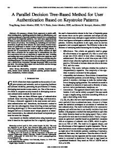
A CCP tree is a compressed representation of the input data. It can be constructed by reading the data sets one transaction at a time and mapping each transaction onto a path in the tree. Since different transactions may have common items, their paths may overlap. Fig. 1 shows a CCP tree constructed by using the datasets in Table 1. Each node N in the CCP tree contains an ordered set of items. Suppose we have m items in node N , then each node can be denoted as N.items[i], i = 1, ..., m. Each item has 6 fields: items.name, item.countD1, item.countD2, item.countS1, item.countS2 and item.child. In the field of an item, item.name records the item name; item.countD1, item.countD2, item.countS1 and item.countS2 are the count of the item in datasets D1 , D2 , S1 and S2 respectively; pointer item.child stores all the children nodes of the current item. The root of the CCP tree is also a node that contains items, which is different from the null root for an FP tree.

4.2. Construction of a CCP tree To illustrate the process of constructing a CCP tree, we use the example provided in Table 1.

Figure 1. CCP tree of the example data set

(i) Datasets D1 and D2 are scanned once to determine the support count of each singleton item. Infrequent items can be discarded in this process. The remaining items are sorted in descending order of support counts, and the item names and support information are stored in a header table. If we set the minimum support to 1.0, we can obtain the ordered item list: b : 6 → a : 5 → d : 3 → c : 2. (ii) The second pass is made to construct the CCP tree. For example, for the case in Table 1, we have the first transaction in D1 , {b, c}. We first sort each transaction by the ordered item list. In this case, it is still {b, c}. Then a node with one item {b, 1, 0, 0, 0, p.child} is created as the root node, and a node with item {c, 1, 0, 0, 0, {}} is stored as the child node of item b. For the second transaction in D1 , we scan the current tree to check if there is an existing path. Because the root node already contains item b, we only increase its field countD1, i.e., the node is updated to {b, 2, 0, 0, 0, p.child}. For transaction {a, b}, it can be sorted as {b, a}. Similarly, item b in the root node is updated to {b, 3, 0, 0, 0, p.child}, and this time, item a is added to the children of item b, which means that item b has a new child item {a, 1, 0, 0, 0, {}}. For the last transaction {d}, since there is no d in the root node, the root node has a new item {d, 1, 0, 0, 0, {}}. This scanning process continues until every transaction in datasets D1 , D2 , S1 and S2 has been mapped onto one of the paths in the CCP tree. The final CCP tree is shown in Fig. 1, and the pseudo code is shown in Algorithm 1 and Algorithm 2.

4.3. Mining CCPs After building the CCP tree, we mine CCPs from the tree. To obtain the count of each itemset, we propose to use the merging subtree algorithm, which is inspired by [3]. The main idea is that the subtree of the current item should be merged with the tree where the current item is located before we decide whether an itemset is a CCP. For example, before we check whether {b} is a CCP or not, we need to merge b’s subtree N to the original tree T . We check all the itemsets using a Depth First Search (DFS) strategy. This means that after checking {b}, we need to check itemset {b, a} (list order is b → a → d → c). Because item {a}’s subtree is not empty, its subtree should be merged with tree N. Thus,

Algorithm 1: create tree(D1 , D2 , S1 , S2 , minsupp ) Input: All the datasets and minimum support threshold of D2 Output: The final CCP tree T = {}; for trans in D2 do count the frequency of each singleton item; delete item in D2 with frequency lower than minsup ; sort remaining items; for trans in D1 , D2 , S1 and S2 do sort trans; insert tree(trans, T ); return T Algorithm 2: insert tree(P , T ) Input: One sorted transaction P ; T is a CCP tree Output: The updated pattern tree T search T for T.item[i] = P [0]; if T.item[i] is not found then insert p at the appropriate place in T obeying the order, denoted as T.item[i]; T.item[i].countD1 = 0; T.item[i].countD2 = 0; T.item[i].countS1 = 0; T.item[i].countS2 = 0; increase T.item[i].countD1, countD2, countS1, DountS2 by 1 according to the class label of the instance; if P [1 :] is not empty then if T.item[i]’s subtree is empty then create a new node N as T.item[i]’s subtree; let N ← T.item[i]’s subtree; call insert tree(P [1 :], N );

for all the itemsets including item b, the order of checking should be {b}, {b, a}, {b, a, d}, {b, a, d, c}, {b, d}, {b, d, c} and {b, c} in our case, as shown in Fig. 2. The pseudo code of merge tree is shown in Algorithm 4. For every item in the header table, if we find it in the current root node of the tree and it has a subtree, merge its subtree into the current tree. Then we add the item to an accumulation itemset β = α ∪ T.item[i], which records the itemset we are checking. If the item satisfies our CCP conditions, the itemset β is a CCP. Then we keep searching its subtree if the item satisfies the first condition C1 and its subtree is not empty. Here, we use condition C1 to decide whether to check the superset of itemsets, because condition C1 is anti-monotone. If β does not satisfy the minimum support threshold, neither will its superset. The algorithm stops when all items in the header table have been checked. The final merged tree is shown in Fig. 2, from which we can see that the counts of all the itemsets are consistent with the statistics of the counts of all possible itemsets shown in Table 2. Here we set minsupp = 1, mingrowth = 2, minratio = 2. This consistency demonstrates that by using our method, we can obtain the correct counts of each item-

set. After applying our conditions, we derive 10 CCPs from all the itemsets. They are {a}, {a, b, d}, {a, b, d, c}, {a, b, c}, {a, d}, {a, d, c}, {a, c}, {b, d}, {b, d, c} and {d}. We can see that pattern {c, d} is a jumping emerging pattern in the transaction dataset, while it is not a conditional contrast pattern, since it does not satisfy condition C3. Algorithm 3: mine tree (T , α, minsupp , mingrowth , minratio , headerT able) Input: T is a pattern tree, α is an accumulating itemset, minsupp , mingrowth and minratio are the minimum support, minimum growth rate, and minimum ratio, which are designed by the user, headerT able stores the sorted singleton item list Output: A set of CCPs for item in headerT able do if item is found in T ’s items T.item[i] then if T.item[i]0 s subtree M is not empty then merge tree(M , T ); β = α ∪ T.item[i]; if T.item[i] satisfies CCP conditions then generate an CCP β of D2 ; if T.item[i]’s subtree N is not empty and T.item[i].countD2 ≥ minsupp then mine tree(N , β , minsupp , mingrowth , minratio , headerT able);

Algorithm 4: merge tree(T 1, T 2) Input: T 1 and T 2 are two pattern trees Output: An updated tree T 2 after being merged with T1 for each item of T 1, T 1.item[i] do search T 2 for T 2.item[j] = T 1.item[i]; if T 2.item[j] is found then update T2.item[j] by adding the count of T1.item[i] correspondingly; else copy and insert T 1.item[i] with its counts and child node at the right place in T 2, and denoted as T 2.item[j]; continue; if T 1.item[i]’s subtree M is not empty then if T 2.item[j]’s subtree is empty then create a new node N as T 2.item[j]’s subtree; N ← T 2.item[j]’s subtree; call merge tree(M ,N );

4.4. Analytical Results 4.4.1. Space complexity. During runtime, we not only need to store the counts of each node, but also the pointers

TABLE 2. C OUNTS OF ALL ITEMSETS OF FOUR DATASETS

D1 D2 S1 S2

a

b

c

d

ab ac ad bc bd cd abc abd acd bcd abcd

1 4 1 1

3 3 2 3

1 1 2 2

1 2 1 1

1 3 0 1

0 1 0 0

0 2 0 0

1 1 1 1

0 2 1 0

0 1 0 1

0 1 0 0

0 2 0 0

0 1 0 0

0 1 0 0

0 1 0 0

Figure 2. Final merged tree of the illustrative dataset

between nodes. This may result in increased storage. To solve this problem, we can adopt the method proposed in [3] and [6], which partitions the data set into a set of projected data sets and mine patterns for each projected dataset. 4.4.2. Computational complexity. A detailed analysis of the time complexity for the CCP tree based algorithm is shown below. Construction of CCP tree: First, we need to scan all the datasets once to obtain the header table. In the second scan, for each transaction, we need to find the right position for each item in the transaction to insert in the current CCP tree. Assuming that Nt is the total number of transactions, w is the average transaction width, and the algorithm complexity of sorting items is O(w · log(w)), then the computational complexity of constructing the CCP tree is O(w·log(w)Nt ). Mining CCPs: The best case happens when all the transactions have the same set of items, which means the CCP tree contains only a single branch of nodes. If all the candidates satisfy the CCP conditions, the algorithm complexity will be O(2w ). In the worst case, all the possible itemsets appear in the transactions and their counts are all greater than the minimum support threshold. In this case, we build the biggest CCP tree. Assuming that d is the number of singleton items, the computational complexity of mining CCPs is O(d · 2d−1 ) in the worst case. This can be derived from the recurrence relation below: F (d) = 2F (d − 1) + 2d−1 for d > 1, F (1) = 1. In practice, since not all the patterns will exist in transactions and not all the patterns satisfy condition C1, the computational complexity will be lower than the worst case O(d · 2d−1 ). 4.4.3. Completeness proof. The construction of the CCP tree is exhaustive, and all the counts in different datasets are recorded in the tree node. This preserves complete information for CCP mining. By merging the tree, we can

obtain the exact counts for each itemset. In our mining algorithm, all possible itemsets are checked except some itemsets that may be pruned by using condition C1, since this condition is anti-monotone. We also test the accuracy of our method using a brute-force method, which checks all combinations of items. The experiments show that the results of these two methods are the same.

5. Performance Evaluation In this section, we evaluate the performance of our CCP tree based method. We describe the synthetic and the real life dataset in Section 5.1, and baseline methods in Section 5.2. Then we compare our method with other methods in terms of efficiency and quality for synthetic data in Section 5.3. In the last section, we show the results derived from the real dataset. All experiments are performed on a laptop with 2.6 R CoreTM i7 − 5600U CPU, 16 GB memory, and GHz Intel Windows 7 64bit Enterprise operating system. The programs are coded in Python (version 3.6.0).

5.1. Synthetic dataset For synthetic data, we simulate a store with Np zones in terms of the product categories. Suppose that we have five categories of customers, who have different probabilities in buying different products. Note that costumers may visit a set of zones and purchase several categories. The probability of a customer belonging to category j buying products in zone i is Pb (i, j), which is chosen arbitrarily, and the value chosen has no effect on the evaluation of our algorithm. The chance that a customer of category j entered zone i, Pv (i, j) is decided by a sale ratio, Ratio, namely: Pv (i, j) = Pb (i, j) · Ratio,

wherein Ratio(j) ≥ 1. Then we can get the probabilities of customers visiting different areas according to the formula above. We also suppose that the probabilities of different categories of customers P (Cate(j)) are equal. For example, if there are 5 categories of customers, P (Cate(j)) = 0.2 for j = 1, ..., 5. By changing the parameter Ratio, we can generate dataset D and S of two different time periods. For example, setting Ratio = 1.1, we can generate dataset D1 and S1 . Similarly, setting Ratio = 1.2, we can generate another two datasets D2 and S2 .

5.2. Real dataset – Melbourne retail shop In this dataset, 78 days of transaction data and spatial data in one store located in Melbourne were collected from November 2015 to February 2016. In the store, a set of sensors are installed, which monitor the position of individual customers over time by detecting the WiFi MAC address of a customer’s mobile phone. Note that some customers may not have a mobile phone, or WiFi is not activated on

their phones. We assume that the proportion of this kind of customer is constant among different days. Since in our problem, we only pay attention to the change of the number of customers, these customers in constant proportion will have no effect on our results. Each trajectory represents one customer visiting the store, and each transaction means one customer buying product(s) in the store. Based on the category of items on the shelf, the store is divided into eight polygon zones, with the cashier zone excluded. The trajectory of one customer is composed of a sequence of 2D points with a unique WiFi MAC address. Based on which zone each 2D point occurs in, each trajectory is translated to a set of zones. Then, a threshold of total dwell time (30 seconds in the current case) is applied to discard customers with a short dwell time. Also, trajectories that occurred out of business hours are considered as those generated by staff, which are removed. Transaction data with a negative amount indicates a refund, which should not be taken into account in our experiment. In all, there are 215, 748 valid trajectories and 109, 752 valid transactions. The name and detailed layout of the store cannot be revealed for confidentiality reasons. The names of the 8 zones in the store are also anonymised.

5.3. Evaluation 5.3.1. Baseline mining methods. We compare our proposed method with two other methods: brute-force method, and Apriori-based method. The brute-force method considers all the combinations of items. It scans the datasets every time it calculates the counts of all the itemsets. Since the first proposed condition satisfies the anti-monotone property, we can apply the Apriori principle to help us reduce the number of possible candidate itemsets. 5.3.2. Results for synthetic data. To evaluate the efficiency of our method, we compared the running time of the three approaches. Fig. 3 shows the running time of the three methods as the number of transactions in each dataset varied from 100 to 20, 000. Other parameters setting are: Np = 15, minsupp = 2, mingrowth = 2, minratio = 2. We can see that the running time of brute-force method increased dramatically as the number of transactions increases. Here, we only provide the results of Brute-force with less than 3000 transactions. When the number of transactions is below 3000 transactions, the Apriori-based method has comparable run time to the CCP-tree based method. However, as the number of transactions further increases, the Aprioribased method becomes slower, while the running time of our proposed method stays almost stable. We also compared the number of patterns we can find using the CCP-tree based method and CP-tree based method [3]. The numbers of CPs and CCPs are also shown in Fig. 3 as the number of transactions in each dataset increased from 100 to 20, 000. We can see that the number of CCPs are less than the number of CPs, since we filter CCPs from CPs by utilizing information from other datasets. The growth rate of the number of CCPs is also slower than CPs. This is

(a) Running time comparison Figure 3. CCP mining time v.s. number of transactions of synthetic data

(b) Number of CCPs and CPs Figure 5. Results on real data - transaction data and spatial data of customers Figure 4. number of CCP and CP v.s. number of transactions of synthetic data

because as the number of transactions increased, there would be more patterns that satisfy the conditions of CPs, while for CCPs, the number of transactions has little influence on the number of CCPs we can find. Table 3 shows the running time of the three methods as the number of items varies. Here the number of transactions in each dataset is 3000. The brute-force method is still the slowest. With only 15 items, its running time can be 61 times longer than the other two methods. When the number of items is no more than 20, the Apriori-based method is a little faster than the CCP-tree based method. While when the number of items reached 25, the CCP-tree based method is about 1.5 times faster than the Apriori-based method. 5.3.3. Results for Melbourne retail shop. In a retail environment, emerging patterns of purchased items are often analyzed to provide sales strategies. Intuitively, sale increases relate to more customer visits. It is the patterns whose sales change significantly but with little variation in customer visits that are of special interest. These patterns fit well with our proposed conditional contrast patterns (CCPs), and can TABLE 3. RUNNING TIME DEPENDING ON THE NUMBER OF ITEMS ON SYNTHETIC DATA

Brute-force Apriori CCP tree

Running time(s) 15 items 20 items 25 items 371.98 5.95 94.67 1384.49 6.08 95.24 986.83

TABLE 4. D ESCRIPTION OF THE FIVE TESTS ON REAL DATA : T RANSACTION DATA AND SPATIAL DATA OF CUSTOMERS Test 1 2 3 4 5

Data Negative 26/12/1528/12/15 25/01/1631/01/16 Sundays Sundays Tuesdays

set Positive 22/12/1524/12/15 01/02/1607/02/16 Mondays Saturdays Mondays

Number of Transactions D1 D2 S1 S2 2,397

7,366

4,706

8,340

9,910

12,195 19,754 29,372

18,129 19,156 34,566 36,965 18,129 18,852 34,566 35,300 17,147 19,156 33,281 36,965

be obtained using our CCP tree based mining algorithm. We select 5 representative time periods from the data to test the performance of our algorithm. The first time periods in comparison are 26/12/2015 − 28/12/2015 and 22/12/2015 − 24/12/2015, which are 3 days after the Christmas Day and 3 days before it. The second comparison are 01/02/2016 − 07/02/2016 and 25/01/2016 − 31/01/2016, which are one week before the start of school and one week after it. The last three comparisons are Sundays and Mondays, Sundays and Saturdays, and Mondays and Tuesdays. The description of the time period is shown in Table 4. Then we obtain five sets of datasets {D = D1 ∪D2 , S = S1 ∪ S2 }. The detailed numbers of transactions in D1 , D2 , S1 and S2 are shown in Table 4. In these experiments, the parameter threshold settings are minsupp = 5, mingrowth = 2, minratio = 2. The running time of the three methods is shown in Fig. 5a. As shown in Fig. 5a, in all the five tests, the running time of Brute-force is the highest, and it strongly depends

on the number of transactions. The Apriori-based method is much better than Brute-force, but it also depends on the number of transactions. Our method is the fastest, with all the running times less than 0.5 second, and the number of transactions has little influence on its performance. The number of CCPs and CPs are shown in Fig. 5b. We can see that the number of CCPs is less than CPs, which means that we extract fewer contrast patterns by utilizing two kinds of datasets and these patterns are more informative and actionable for decision makers. We also notice that in test 1 and test 2, although the number of transactions is less than the number of transactions in test 3, test 4 and test 5, the number of CCPs in the first two cases is larger than the number in the last three cases. This means that the time periods under contrast are more different than other time periods.

6. Conclusion In this paper, we have introduced a new kind of contrast pattern, conditional contrast patterns. In contrast to normal contrast patterns, CCPs are able to use information from other data sources. We also have proposed a conditional contrast pattern tree based algorithm for mining CCPs. By comparing our method with two other baseline methods (brute-force method and Apriori-based method) on synthetic data, we have evaluated the efficiency of our method. The results show that our CCP tree based method is the most efficient one among these methods. A real world case study relating to customer behaviours has been applied to further explain our proposed method. Overall, we believe that we have proposed a useful and interesting contrast pattern for multi-source mining, and our proposed CCP method is practical in analysing data from retail environments. Also, we believe CCPs can be applied to other areas, such as classification. In the future, we would like to develop more time efficient methods, such as approximate methods, for mining CCPs.

[4] Elsa Loekito, and James Bailey, ”Fast mining of high dimensional expressive contrast patterns using zero-suppressed binary decision diagrams.” in Proceedings of the 12th ACM SIGKDD International Conference on Knowledge Discovery and Data Mining, pp. 307-316. 2006. [5] Garc´ıa-Borroto Milton, Jos´e Fco Mart´ınez-Trinidad, and Jes´us Ariel Carrasco-Ochoa, ”Fuzzy emerging patterns for classifying hard domains.” Knowledge and Information Systems, 28(2), pp. 473-489. 2011. [6] Jiawei Han, Jian Pei, Yiwen Yin, and Runying Mao, ”Mining frequent patterns without candidate generation: A frequent-pattern tree approach.” Data Mining and Knowledge Discovery, 8(1), pp. 53-87. 2004. [7] Jinyan Li, Ramamohanarao Kotagiri, and Guozhu Dong, ”The Space of Jumping Emerging Patterns and Its Incremental Maintenance Algorithms.”, in Proceedings of International Conference on Machine Learning, pp. 551-558. 2000. [8] Xiaoting Wang, Christopher Leckie, Hairuo Xie, and Tharshan Vaithianathan, ”Discovering the impact of urban traffic interventions using contrast mining on vehicle trajectory data.”, in Pacific-Asia Conference on Knowledge Discovery and Data Mining, pp. 486-497. 2015. [9] Jae-Gil Lee, Jiawei Han, Xiaolei Li, and Hong Cheng, ”Mining discriminative patterns for classifying trajectories on road networks.” IEEE Transactions on Knowledge and Data Engineering, 23(5), pp. 713-726. 2011. [10] Bin Shen, Qiuhua Zheng, Xingsen Li, and Libo Xu, ”A framework for mining actionable navigation patterns from in-store RFID datasets via indoor mapping.” Sensors, 15(3), pp. 5344-5375. 2015. [11] Li Li, and Christopher Leckie, ”Trajectory Pattern Identification and Anomaly Detection of Pedestrian Flows Based on Visual Clustering.” in Proceedings of the 12th International Conference on Intelligent Information Processing, pp. 121-131. 2016. [12] Yaeli Avi, Peter Bak, Guy Feigenblat, Sima Nadler, Haggai Roitman, Gilad Saadoun, Harold J. Ship et al, ”Understanding customer behavior using indoor location analysis and visualization.” IBM Journal of Research and Development, 58(5/6), pp. 3-1. 2014. [13] Chao Gao, Lei Duan, Guozhu Dong, Haiqing Zhang, Hao Yang, and Changjie Tang, ”Mining Top-k Distinguishing Sequential Patterns with Flexible Gap Constraints.” in Proceedings of International Conference on Web-Age Information Management, pp. 82-94. 2016. [14] Yu Zheng, Licia Capra, Ouri Wolfson, and Hai Yang, ”Urban computing: concepts, methodologies, and applications.” ACM Transactions on Intelligent Systems and Technology (TIST), 5(3), pp. 38. 2014.

Acknowledgments

[15] Dong Guozhu, and James Bailey, eds. Contrast Data Mining: Concepts, Algorithms, and Applications. Chapman and Hall/CRC, 2012.

The authors want to acknowledge the anonymous reviewers for their constructive suggestions and feedback.

[16] Xiangtao Chen, and Lijuan Lu, ”A new algorithm based on shared pattern-tree to mine shared emerging patterns.” in Proceedings of the IEEE 11th International Conference on Data Mining Workshops, pp. 1136-1140. 2011.

References

[17] Jixian Zhang, ”Multi-source remote sensing data fusion: status and trends.” International Journal of Image and Data Fusion, 1(1), pp. 5-24. 2010.

[1] Stephen D. Bay, and Michael J. Pazzani, ”Detecting change in categorical data: Mining contrast sets.” in Proceedings of the Fifth ACM SIGKDD International Conference on Knowledge Discovery and Data Mining, pp. 302-306. 1999.

[18] Ramkumar Thirunavukarasu, Shanmugasundaram Hariharan, and Shanmugam Selvamuthukumaran, ”A survey on mining multiple data sources.” Wiley Interdisciplinary Reviews: Data Mining and Knowledge Discovery, 3(1), pp. 1-11. 2013.

[2] Guozhu Dong, and Jinyan Li, ”Efficient mining of emerging patterns: Discovering trends and differences.” in Proceedings of the Fifth ACM SIGKDD International Conference on Knowledge Discovery and Data Mining, pp. 43-52. 1999. [3] Hongjian Fan, and Ramamohanarao Kotagiri, ”Fast discovery and the generalization of strong jumping emerging patterns for building compact and accurate classifiers.” IEEE Transactions on Knowledge and Data Engineering, 18(6), pp. 721-737. 2006.