semi-definite (PSD) matrices whose eigenvalues are non- negative ... different approaches to transforming a non-PSD matrix into a PSD ..... to make KEros PSD}.
A PCA-based Kernel for Kernel PCA on Multivariate Time Series Kiyoung Yang and Cyrus Shahabi Computer Science Department University of Southern California Los Angeles, CA 90089-0781 [kiyoungy,shahabi]@usc.edu
Abstract Multivariate time series (MTS) data sets are common in various multimedia, medical and financial application domains. These applications perform several data-analysis operations on large number of MTS data sets such as similarity searches, feature-subset-selection, clustering and classification. Inherently, an MTS item has a large number of dimensions. Hence, before applying data mining techniques, some form of dimension reduction, e.g., feature extraction, should be performed. Principal Component Analysis (PCA) is one of the techniques that have been frequently utilized for dimension reduction. However, traditional PCA does not scale well in terms of dimensionality, and therefore may not be applied to MTS data sets. The Kernel PCA technique addresses this problem of scalability by utilizing the kernel trick. In this paper, we propose a PCA based kernel to be employed for the Kernel PCA technique on the MTS data sets, termed KEros, which is based on Eros, a PCA based similarity measure for MTS data sets. We evaluate the performance of KEros using Support Vector Machine (SVM), and compare the performance with Kernel PCA using linear kernel and Generalized Principal Component (GPCA). The experimental results show that KEros outperforms these other techniques in terms of classification accuracy.
1 INTRODUCTION A time series is a series of observations, xi (t); [i = 1, · · · , n; t = 1, · · · , m], made sequentially through time where i indexes the measurements made at each time point t [20]. It is called a univariate time series (UTS) when n is equal to 1, and a multivariate time series (MTS) when n is equal to, or greater than 2. A UTS data is usually represented in a vector of size m, while each MTS item is typically stored in an m × n matrix, where m is the number of observations and n is the number of variables (e.g., sen-
sors). MTS data sets are common in various fields, such as in multimedia, medicine and finance. For example, in multimedia, Cybergloves used in the Human and Computer Interface (HCI) applications have around 20 sensors, each of which generates 50∼100 values in a second [11, 19]. For gesture recognition and video sequence matching using computer vision, several features are extracted from each image continuously, which renders them MTSs [5, 2, 17]. In medicine, Electro Encephalogram (EEG) from 64 electrodes placed on the scalp are measured to examine the correlation of genetic predisposition to alcoholism [26]. Functional Magnetic Resonance Imaging (fMRI) from 696 voxels out of 4391 has been used to detect similarities in activation between voxels in [7]. An MTS item is typically very high dimensional. For example, an MTS item from one of the data sets used in the experiments in Section 4 contains 3000 observations with 64 variables. If a traditional distance metric for similarity search, e.g., Euclidean Distance, is to be utilized, this MTS item would be considered as a 192000 (3000 × 64) dimensional data. 192000 dimensional data would be overwhelming not only for the distance metric, but also for indexing techniques. To the best of our knowledge, there has been no attempt to index data sets with more than 100000 dimensions/features1 . Hence, it would be necessary to preprocess the MTS data sets and reduce the dimension of each MTS item before performing any data mining tasks. A popular method for dimension reduction is Principal Component Analysis (PCA) [10]. Intuitively, PCA first finds the direction where the variance is maximized and then projects the data on to that direction. However, traditional PCA cannot be applied to MTS data sets as is, since each MTS item is represented in a matrix, while for PCA each item should be represented as a vector. Though each MTS item may be vectorized by concatenating its UTS items (i.e., the columns of MTS), this would result in the 1 In [3], the authors employed MVP-tree to index 65536 dimensional gray-level MRI images.
Symbol A AT MA VA
loss of the correlation information among the UTS items. In order to overcome this limitation of PCA, i.e., the data should be in the form of a vector, Generalized Principal Component Analysis (GPCA) is proposed in [24]. GPCA works on the matrices and reduces the number of rows and columns simultaneously by projecting a matrix into a vector space that is the tensor product of two lower dimensional vector spaces. Hence the data do not need to be vectorized. While GPCA reduces the dimension of an MTS item, the reduced form is still a matrix. In order to be fed into such data mining techniques as Support Vector Machine (SVM) [21], the reduced form still needs to be vectorized, which would be a whole new challenge. Moreover, for traditional PCA, even if each MTS item is vectorized, the space complexity of PCA would be overwhelming. For example, assume an MTS item with 3000 observations and 64 variables. If this MTS item is vectorized by concatenating each column end to end, the length of the vector would be 192000. Assume that there are 378 items in the data set. Then the whole data set would be represented in a matrix of size 378 × 192000. Though, in theory, the space complexity of PCA is O(nN ) where n is the number of features/dimensions and N is the number of items in the data set [14], Matlab fails to perform PCA on a matrix of size 378 × 192000 on a machine with 3GB of main memory due to lack of memory. In [8], it has also been observed that PCA does not scale well as a function of dimensionality. In [18], the authors proposed an extension of PCA using kernel methods, termed Kernel PCA. Intuitively, what the Kernel PCA does is firstly to transform the data into a high dimensional feature space using a possibly non-linear kernel function, and then to perform PCA in the high dimensional feature space. In effect, Kernel PCA computes the pair-wise distance/similarity matrix of size N × N using a kernel function, where N is the number of items. This matrix is called a Kernel Matrix. Kernel PCA therefore scales well in terms of dimensionality of the data, since the kernel function can be efficiently computed using the Kernel Trick [1]. Depending on the kernel employed, Kernel PCA has been shown to yield better classification accuracy using the principal components in feature space than in input space. However, it is an open question which kernel is to be used [18]. In this paper, we propose to utilize Eros [22] for the Kernel PCA technique, termed KEros. By using Eros, the data need not be transformed into a vector for computing the similarity between two MTSs, which enables us to capture the correlation information among the UTSs in an MTS item. In addition, by using the kernel technique, the scalability problem in terms of dimensionality is resolved. KEros firstly computes a matrix that contains pair-wise similarities between MTSs using Eros, and utilizes this matrix as
ΣA ai aij a∗j w
Definition an m × n matrix representing an MTS item the transpose of A the covariance matrix of size n × n for A the right eigenvector matrix of size n × n for MA VA = [ a1 , a 2 , · · · , a n ] an n × n diagonal matrix that has all the eigenvalues for MA obtained by SVD a column orthonormal eigenvector of size n for VA jth value of ai , i.e., a value at the ith column and the jth row of A all the values at the jth row of A a weight vector of size n P r w = 1, ∀i wi ≥ 0 i=1 i
Table 1. Notations used in this paper the Kernel Matrix for the kernel PCA technique. Though Eros cannot readily be formulated in terms of dot product as other kernel functions, it has been shown that any positive semi-definite (PSD) matrices whose eigenvalues are nonnegative can be utilized for kernel techniques [13]. If the matrix obtained by using Eros is shown to be positive semidefinite, it can be utilized as a Kernel Matrix as is; otherwise, the matrix can be transformed into a Kernel Matrix by utilizing one of the techniques proposed in [16]. In this paper, we utilize the first na¨ıve approach. We plan to compare different approaches to transforming a non-PSD matrix into a PSD matrix for Eros in the future. In order to evaluate the effectiveness of the proposed approach, we conducted experiments on two real-world data sets: AUSLAN [11] obtained from UCI KDD repository [9] and the Brain Computer Interface (BCI) data set [12]. After performing dimension reduction using KEros, we compared the classification accuracy with other techniques, such as Generalized Principal Component Analysis (GPCA) [24], and Kernel PCA using linear kernel. The experimental results show that KEros outperforms other techniques by up to 60% in terms of classification accuracy. The remainder of this paper is organized as follows. Section 2 discusses the background of our proposed approach. Our proposed approach is presented in Section 3, which is followed by the experiments and results in Section 4. Conclusions and future work are presented in Section 5.
2 BACKGROUND Our proposed approach is based on Principal Component Analysis (PCA) and our similarity measure for Multivariate Time Series (MTS), termed Eros. In this section, we briefly describe PCA and Eros. For details, please refer to [10, 22]. For notations used in the remainder of this paper, please refer to Table 1. 2
In practice, PCA is performed by applying Singular Value Decomposition (SVD) to either a covariance matrix or a correlation matrix of an MTS item depending on the data set. That is, when a covariance matrix A is decomposed by SVD, i.e., A = U ΛU T , a matrix U contains the variables’ loadings for the principal components, and a matrix Λ has the corresponding variances along the diagonal [10].
X2 PC 1 = (cosa 1 )X 1 + (cosß 1 )X2 ß1
a1 X1
2.2 Score (Orthogonal Projection)
In [22], we proposed Eros as a similarity measure for multivariate time series. Intuitively, Eros computes the similarity between two matrices using the principal components (PCs), i.e., the eigenvectors of either the covariance or the correlation coefficient matrices, and the eigenvalues as weights. The weights are aggregated from the eigenvalues of all the MTS items in the database. Hence, the weights change whenever data are inserted into or removed from the database.
Figure 1. Two principal components obtained for one multivariate data with two variables x1 and x2 measured on 30 observations.
2.1
Eros
PC 2
Principal Component Analysis
Definition 1 Eros (Extended Frobenius norm). Let A and B be two MTS items of size mA × n and mB × n, respectively2 . Let VA and VB be two right eigenvector matrices obtained by applying SVD to the covariance matrices, MA and MB , respectively. Let VA = [a1 , · · · , an ] and VB = [b1 , · · · , bn ], where ai and bi are column orthonormal vectors of size n. The Eros similarity of A and B is then defined as Pn Pn Eros(A,B,w)= wi ||= wi | cos θi | (1) i=1 i=1
Principal Component Analysis (PCA) has been widely used for multivariate data analysis and dimension reduction [10]. Intuitively, PCA is a process to identify the directions, i.e., principal components (PCs), where the variances of scores (orthogonal projections of data points onto the directions) are maximized and the residual errors are minimized assuming the least square distance. These directions, in non-increasing order, explain the variations underlying original data points; the first principal component describes the maximum variation, the subsequent direction explains the next maximum variance and so on. Figure 1 illustrates principal components obtained on a very simple (though unrealistic) multivariate data with only two variables (x1 , x2 ) measured on 30 observations. Geometrically, the principal component is a linear transformation of original variables and the coefficients defining this transformation are called loadings. For example, the first principal component (PC1) in Figure 1 can be described as a linear combination of original variables x1 and x2 , and the two coefficients (loadings) defining PC1 are the cosines of the angles between PC1 and variables x1 and x2 , respectively. The loadings are thus interpreted as the contributions or weights on determining the directions. The central idea of principal component analysis (PCA) is to reduce the dimensionality of a data set consisting of a large number of interrelated variables, while retaining as much as possible the variation present in the data set [10]. This is achieved by transforming to a new set of variables, the principal components (PCs), which are uncorrelated, and which are ordered so that the first few retain most of the variation present in all of the original variables.
where < ai , bi > is the inner product of ai and bi , w is a weight vector Pn which is based on the eigenvalues of the MTS data set, i=1 wi = 1 and cos θi is the angle between ai and3 bi . The range of Eros is between 0 and 1, with 1 being the most similar. Intuitively, each wi in the weight vector represents the aggregated variance for all the ith principal Pn components. The weights are then normalized so that i=1 wi = 1. The eigenvalues obtained from all the MTS items in the database are aggregated into one weight vector as in Algorithms 1 or 2. Algorithm 1 computes the weight vector w based on the distribution of raw eigenvalues, while Algorithm 2 first normalizes each si , and then calls Algorithm 1. Function f () in Line 3 of Algorithm 1 is an aggregating function, e.g., min, mean and max. Note that PCA, on which Eros is based, may be described as firstly representing each MTS item using either 2 MTS items have the same number of columns (e.g., sensors), but may have different number of rows (e.g., time samples). 3 For simplicity, it is assumed that the covariance matrices are of full rank. In general, the summations in Equation (1) should be from 1 to min(rA , rB ), where rA is the rank of MA and rB the rank of MB .
3
Algorithm 1 Computing a weight vector w based on the distribution of raw eigenvalues 1: function computeWeightRaw(S) Require: an n×N matrix S, where n is the number of variables for the dataset and N is the number of MTS items in the dataset. Each column vector si in S represents all the eigenvalues for ith MTS item in the dataset. sij is a value at column i and row j in S. s∗i is ith row in S. si∗ is ith column, i.e, si . 2: for i=1 to n do 3: wi ← f (s∗i ); 4: end for 5: for i=1 to n do Pn 6: wi ← wi / j=1 wj ; 7: end for
achieved by solving the following eigenvalue problem: λv = Cv
Kernel PCA extends this traditional PCA approach, and performs PCA in the feature space. Hence, the data are first mapped into a high dimensional feature space using Φ : RN → F, x 7→ X. The covariance matrix in the feature space can be described as follows, assuming that data are centered: N 1X Φ(xi )Φ(xi )T C= N i=1 An N × N Kernel Matrix, which is also called as Gram matrix, can be defined as follows: Kij = (Φ(xi ) · Φ(xj )) = k(xi , xj )
Algorithm 2 Computing a weight vector w based on the distribution of normalized eigenvalues 1: function computeWeightRatio(S) Require: the same as Algorithm 1. 2: for i=1 to N do Pn 3: si ← si / j=1 sij ; 4: end for 5: computeWeightRaw(S);
and as Equation (2), one computes an eigenvalue problem for the expansion coefficients αi , that is now solely dependent on the kernel function λα = Kα
(3)
Hence, intuitively, Kernel PCA can be performed by firstly obtaining the Kernel Matrix, and then solving the eigenvalue problem as in Equation (3). For details, please refer to [18, 15]. Let us formally define the kernel function and the kernel matrix [13].
covariance or correlation coefficients, and then performing SVD on the matrix that contains the coefficients. In order to stably represent an MTS using correlation coefficients, we proposed to utilize the stationarity of time series before computing the correlation coefficients of an MTS item [23]. Intuitively, if a time series is stationary, it means that the statistical properties of a time series, e.g., covariance and correlation coefficients, do not change over time. For details, please refer to [23].
Definition 2 A kernel is a function k, such that k(x, z) = < Φ(x), Φ(z) > for all x, z ∈ X , where Φ is a mapping from X to an (inner product) feature space F . A kernel matrix is a square matrix K ∈ RN ×N such that Kij = k(xi , xj ) for some x1 , · · · , xN ∈ X and some kernel function k. As in [13], the kernel matrices can be characterized as follows:
3 THE PROPOSED APPROACH
Proposition 1 Every positive semi-definite and symmetric matrix is a kernel matrix. Conversely, every kernel matrix is symmetric and positive semi-definite.
In this section, we will firstly describe the traditional PCA in a little more detail, and then briefly describe the kernel PCA technique in relation to the traditional PCA, which will be followed by our proposed approach. Assume that we are given a set of N items, and each data item is an n dimensional column vector, i.e., xi ∈ Rn , where 1 ≤P i ≤ N . Assume also that the data is mean cenn tered, i.e., i=1 xji = 0, for 1 ≤ j ≤ N . The covariance matrix can subsequently be computed as follows:
As a kernel function for Kernel PCA technique, we propose to utilize Eros for MTS data sets. That is, given an MTS data set X and a weight vector w, the Kernel Matrix is constructed in such a way that K Eros (i, j) = Eros(Xi , Xj , w). Note that Eros is not a distance metric, and cannot be readily represented in a form of dot product as the other kernel functions. However, according to Proposition 1, K Eros can be utilized for Kernel PCA, as long as K Eros is symmetric and positive semi-definite, i.e., the eigenvalues of K Eros is non-negative. Firstly, Eros is symmetric, i.e., Eros(Xi , Xj , w) = Eros(Xj , Xi , w). Hence, K Eros is symmetric. Consequently, as long as K Eros is positive semi-definite, K Eros can be utilized for Kernel
1X xi xTi N i=1 N
C=
(2)
The traditional PCA then diagonalizes the covariance matrix to obtain the principal components, which can be 4
PCA. In [16], a number of approaches to making a matrix into a PSD matrix have been described. In this paper, we utilize the first na¨ıve approach4, which is to add Eros δI to K Eros , i.e., K ← K Eros + δI, when K Eros is not PSD. For δ sufficiently larger in absolute value than the Eros most negative eigenvalue of K Eros , K is PSD. Algorithms 3 and 4 describes how to compute K Eros , and how to obtain the principal components in the feature space. Given an MTS data set, and a weight vector w, we first construct the pair-wise similarity matrix, K Eros , of size N × N , where N is the number items in the given data set as in Lines 2∼7 of Algorithm 3. Lines 8∼10 make sure KEros is PSD. The Kernel Matrix, KEros , is then meancentered in the feature space in Line 3 of Algorithm 4. The eigenvalue problem in the feature space, i.e., the Equation (3), is solved, and the principal components in feature space are obtained in Line 4.
After obtaining the principal components in feature space using the training MTS items as in Algorithms 3 and 4, the projection of the test MTS items on the principal components is performed as in Algorithms 5 and 6. Intuitively, Lines 1∼4 of Algorithm 6 describe how to map the test data into feature space and subtract the pre-computed mean, i.e., mean-center the mapped data in the feature space. Line 5 projects the mean-centered data onto the principal components, V, in the feature space, which is analogous to the traditional PCA approach. For details, please refer to [18]. Algorithm 5 Compute K Eros for Projection Require: MTS data set, X with N {the number of items in the data set} and n {the number of variables in an MTS data}; w {a weight vector for Eros}; MTS data set, Xtest with Ntest and n. 1: {Construct a Kernel Matrix using Eros for Projection} 2: for i = 1 to Ntest do 3: for j = 1 to N do 4: KEros (i, j) ← Eros(Xtest,i , Xj , w); {Xi is the ith MTS item in X, and Xtest,i the ith MTS item in Xtest } 5: end for 6: end for
Algorithm 3 Compute K Eros Require: MTS data set, X with N {the number of items in the data set} and n {the number of variables in an MTS data}; w {a weight vector for Eros} 1: {Construct a Kernel Matrix using Eros} 2: for i = 1 to N do 3: for j = i to N do 4: KEros (i, j) ← Eros(Xi , Xj , w); {Xi is the ith MTS item in X} 5: K(j, i) ← K(i, j); 6: end for 7: end for 8: if KEros is not PSD then 9: KEros ← KEros + δI; {choose sufficiently large δ to make KEros PSD} 10: end if
Algorithm 6 Project Test Data Set using K Eros Require: MTS data set, X with N {the number of items in the data set} and n {the number of variables in an MTS data}; w {a weight vector for Eros}; test MTS data set, Xtest with Ntest and n; V obtained in Algorithm 4 1: KEros test ← Computer the Kernel Matrix using Algorithm 5; 2: KEros ← Computer the Kernel Matrix using Algorithm 3; 3: {Center the Kernel Matrix in feature space} Eros Eros 4: K ← KEros − KEros test − Otest × K test × O + Eros Otest ×K ×O; {where Oij = 1/N, 1 ≤ i, j ≤ N , Otest,ij = 1/N, 1 ≤ i ≤ Ntest , 1 ≤ j ≤ N }
Algorithm 4 Perform PCA using K Eros Require: MTS data set, N {the number of items in the data set}, n {the number of variables in an MTS data}, w {a weight vector for Eros} 1: KEros ← Computer the Kernel Matrix using Algorithm 3; 2: {Center the Kernel Matrix in feature space} Eros 3: K ← KEros − O × KEros − KEros × O + O × Eros K × O; {where Oij = 1/N, 1 ≤ i, j ≤ N and N is the number of items} Eros 4: [V, v] ← solve the eigenvalue problem λα = K α; {V contains the eigenvectors, and v the corresponding eigenvalues}
5:
Eros
Y←K × V; {The ith MTS item is represented as features in the ith row of Y}
4 PERFORMANCE EVALUATION 4.1
Datasets
The experiments have been conducted on two different real-world data sets, i.e., AUSLAN and BCI, which are all labeled MTS data sets whose labels are given. The Aus-
4 We
plan to compare different approaches to transforming a non-PSD matrix into a PSD matrix for Eros in the future.
5
and performing PCA on it to extract the features. GPCA does not require vectorization of the data, and works on each MTS item, i.e., a matrix, to reduce it to a (ℓ1 , ℓ2 ) dimensional matrix. In [24], the best results have been reported when ℓℓ21 = 1. Hence, we varied ℓ1 and ℓ2 from 2 to 7, and the sizes of the reduced matrix would be 4, 9, 16, 25, 36 and 49, respectively. In order to utilize SVM, these reduced matrices have been vectorized column-wise. One of the disadvantages of GPCA and KLinear is that the number of observations within the MTS items should be all the same, while KEros, i.e., Eros, can be applied to the MTS items with variable number of observations. Hence, for GPCA and KLinear, the AUSLAN data set have been linearly interpolated, so that all the items have the same number of observations, which is the mean number of observations, i.e., 60. For KLinear, STPRtool implementation [6] and SVMKM implementation [4] are utilized. For KEros, we modified the Kernel PCA routine in STPRtool and SVM-KM. We implemented GPCA from scratch. All the implementations are written in Matlab.
Table 2. Summary of data sets used in the experiments AUSLAN BCI # of variables 22 64 (average) length 60 3000 # of labels 95 2 # of MTS items per label 27 189 total # of MTS items 2565 378
tralian Sign Language (AUSLAN) data set uses 22 sensors on the hands to gather the data sets generated by signing of a native AUSLAN speaker [11]. It contains 95 distinct signs, each of which has 27 examples. In total, the number of signs gathered is 2565. The average length is around 60. The Brain Computer Interface (BCI) data set [12] was collected during the BCI experiment, where a subject had to perform imagined movements of either the left small finger or the tongue. The time series of the electrical brain activity was collected during these trials using 64 ECoG platinum electrodes. All recordings were gathered at 1000Hz. The total number of items is 378 and the length is 3000. Table 2 shows the summary of the data sets used in the experiments.
4.2
4.3
RESULTS
In order to check if the pair-wise similarity matrix computed by using Eros, i.e., KEros , is positive semi-definite, we obtained the eigenvalues of KEros . For the AUSLAN data set, the minimum eigenvalue of KEros is 3.2259e-06, and for the BCI data set, it is 0.0014. Hence, KEros for the AUSLAN and BCI data sets turned out to be symmetric and positive semi-definite, i.e., all the eigenvalues are non-negative. Consequently, we did not need to add δI to KEros ; for the AUSLAN and BCI data sets, KEros is utilized as is as the Kernel Matrix for the Kernel PCA technique. Figure 2(a) shows the results of the classification accuracy for the AUSLAN data set. Using only 14 features obtained by KEros, the classification accuracy is over 90%. As we increase the number of features for SVM, the performance of KLinear improves and when the number of features is more than 40, the performance difference between KLinear and KEros is almost negligible. The performance of GPCA, however, is much worse than the Kernel PCA technique. Even when 49 features are employed, the classification accuracy is less then 80%, while the others achieved more than 90% of classification accuracy. There may be a couple of reasons for this poor performance of GPCA. Firstly, in [24], the data sets contain images which are represented in approximately square matrices. For the AUSLAN data set, however, each MTS item is not square; the number of observations is almost three times the number of variables. Hence, the ℓ1 and ℓ2 parameters for GPCA should be re-evaluated. Secondly, the result of dimension
Methods
For KEros, we first need to construct KEros . As described in Section 2.2, there are 6 different ways of obtaining weights for Eros. For the data sets used in the experiments, the mean aggregating function on the normalized eigenvalues yields the overall best results, which are presented in this section. In order to compute the classification accuracy of KEros, we performed 10 fold cross validation (CV) employing Support Vector Machine (SVM) [21]. That is, we break an MTS data set into 10 folds, use 9 folds to obtain the principal components in the feature space using KEros and then project the data in the remaining 1 fold onto the first 51 principal components to obtain 51 features. We subsequently computed the classification accuracy varying the number of features from 1 to 51. We repeated the 10 fold cross validation ten times, and report the average classification accuracy. We compared the performance of KEros with two other techniques, Kernel PCA using linear kernel (KLinear), and Generalized Principal Component Analysis (GPCA) [24], in terms of classification accuracy. Since the linear kernel is the simplest kernel for the Kernel PCA technique, we chose the linear kernel as the performance baseline for the Kernel PCA technique. Note that intuitively Kernel PCA using linear kernel would perform similarly to vectorizing an MTS item column-wise, i.e., concatenate columns back to back, 6
100
90
90
80
80 Classification Accuracy (%)
Classification Accuracy (%)
100
70 60 50 40 30 20
70 60 50 40 30 20
KEros KLinear GPCA
10 0
KEros KLinear GPCA
0
10
20
30 # of features
40
10 0
50
5
(a) AUSLAN Dataset
10
15
20
25 30 # of features
35
40
45
50
(b) BCI Dataset
Figure 2. Classification Accuracy Comparison to extract features, the classification accuracy is up to 60% better than using features extracted using linear kernel, and Generalized Principal Component Analysis (GPCA) [24]. We intend to extend this research in two directions. Firstly, more comprehensive experiments with more realworld data sets will be performed including comparisons with other techniques such as Kernel LDA [15]. In [25], we utilized the principal component loadings to identify a subset of variables that are least redundant in terms of contributions to the principal components. We plan to explore similar feature subset selection techniques utilizing kernel methods.
reduction using GPCA is still a matrix; a vectorization is required so that SVM can be utilized. Our vectorization by simply concatenating the columns may have resulted in the loss of correlation information. Figure 2(b) represents the classification accuracies of the three techniques on the BCI data set. Similarly as for the AUSLAN data set, KEros outperforms other techniques in terms of classification accuracy. When 16 features are used, KEros yielded more than 70% of classification accuracy. Unlike for the AUSLAN data set, KLinear does not perform as well as KEros as the number of features increased. 16 features from KLinear achieved just more than 60% of classification accuracy. The performance of GPCA is not good for the BCI data set as well; the classification accuracy is more or less the chance level, i.e., 50%. As described for the AUSLAN data set, the parameters for GPCA seem to require re-configuration for the data sets whose items are not square matrices.
Acknowledgement This research has been funded in part by NSF grants EEC-9529152 (IMSC ERC), IIS-0238560 (PECASE) and IIS-0307908, and unrestricted cash gifts from Microsoft. Any opinions, findings, and conclusions or recommendations expressed in this material are those of the author(s) and do not necessarily reflect the views of the National Science Foundation. The authors would also like to thank the anonymous reviewers for their valuable comments.
5 CONCLUSIONS AND FUTURE WORK In this paper, we proposed a technique to utilize Kernel PCA technique to extract features from MTS data sets using Eros as its similarity measure, termed KEros. Using Eros as a similarity measure between two MTS items, the correlation information between UTSs in one MTS item would not be lost. In addition, utilizing the Kernel Trick, KEros does scale well in terms of dimensionality of data sets. KEros first constructs the pair-wise similarity matrix using Eros, KEros . In order to be utilized as a Kernel Matrix for the Kernel PCA technique, KEros is na¨ıvely transformed, if necessary, in such a way that the transformed KEros is positive semi-definite, i.e., all the eigenvalues of KEros are nonnegative. Our experimental results show that using KEros
References [1] M. Aizerman, E. Braverman, and L. Rozonoer. Theoretical foundations of the potential function method in pattern recognition learning. Automation and Remote Control, 25:821–837, 1964. [2] J. Alon, S. Sclaroff, G. Kollios, and V. Pavlovic. Discovering clusters in motion time-series data. In IEEE Computer Vision and Pattern Recognition, pages 18–20, June 2003. [3] T. Bozkaya and M. Ozsoyoglu. Indexing large metric spaces for similarity search queries. ACM TODS, 24(3), 1999.
7
[23] K. Yang and C. Shahabi. On the stationarity of multivariate time series for correlation-based data analysis. In The Fifth IEEE International Conference on Data Mining, Houston, TX, USA, November 2005. [24] J. Ye, R. Janardan, and Q. Li. Gpca: an efficient dimension reduction scheme for image compression and retrieval. In KDD ’04: Proceedings of the tenth ACM SIGKDD international conference on Knowledge discovery and data mining, pages 354–363, New York, NY, USA, 2004. ACM Press. [25] H. Yoon, K. Yang, and C. Shahabi. Feature subset selection and feature ranking for multivariate time series. IEEE Trans. Knowledge Data Eng. - Special Issue on Intelligent Data Preparation, 17(9), September 2005. [26] X. L. Zhang, H. Begleiter, B. Porjesz, W. Wang, and A. Litke. Event related potentials during object recognition tasks. Brain Research Bulletin, 38(6):531–538, 1995.
[4] S. Canu, Y. Grandvalet, and A. Rakotomamonjy. Svm and kernel methods matlab toolbox. Perception Systmes et Information, INSA de Rouen, Rouen, France, 2003. [5] A. Corradini. Dynamic time warping for off-line recognition of a small gesture vocabulary. In IEEE RATFG, pages 82– 89, July 2001. [6] V. Franc and V. Hlav´acˇ . Statistical pattern recognition toolbox for matlab. http://cmp.felk.cvut.cz/∼xfrancv/stprtool/, June 2004. [7] C. Goutte, P. Toft, E. Rostrup, F. A. Nielsen, and L. K. Hansen. On clustering fMRI time series. NeuroImage, 9(3):298–310, 1999. [8] D. J. Hand, P. Smyth, and H. Mannila. Principles of data mining. MIT Press, Cambridge, MA, USA, 2001. [9] S. Hettich and S. D. Bay. The UCI KDD Archive. http://kdd.ics.uci.edu, 1999. [10] I. T. Jolliffe. Principal Component Analysis. Springer, 2002. [11] M. W. Kadous. Temporal Classification: Extending the Classification Paradigm to Multivariate Time Series. PhD thesis, University of New South Wales, 2002. [12] T. N. Lal, T. Hinterberger, G. Widman, M. Schr¨oder, N. J. Hill, W. Rosenstiel, C. E. Elger, B. Sch¨olkopf, and N. Birbaumer. Methods towards invasive human brain computer interfaces. In Advances in Neural Information Processing Systems 17, pages 737–744. Cambridge, MA, 2005. [13] G. R. G. Lanckriet, N. Cristianini, P. Bartlett, L. E. Ghaoui, and M. I. Jordan. Learning the kernel matrix with semidefinite programming. J. Mach. Learn. Res., 5:27–72, 2004. [14] Q. Li, J. Ye, and C. Kambhamettu. Linear projection methods in face recognition under unconstrained illuminations: a comparative study. In Computer Vision and Pattern Recognition, 2004. CVPR 2004. Proceedings of the 2004 IEEE Computer Society Conference on, volume 2, pages 474–481, July 2004. [15] K.-R. M¨uller, S. Mika, G. R¨atsch, K. Tsuda, and B. Sch¨olkopf. An introduction to kernel-based learning algorithms. IEEE Trans. Pattern Anal. Machine Intell., 12(2):181–201, March 2001. [16] X. Nguyen, M. I. Jordan, and B. Sinopoli. A kernel-based learning approach to ad hoc sensor network localization. ACM Trans. Sen. Netw., 1(1):134–152, 2005. [17] C. Rao, A. Gritai, M. Shah, and T. Syeda-Mahmood. Viewinvariant alignment and matching of video sequences. In IEEE ICCV, pages 939–945, October 2003. [18] B. Sch¨olkopf, A. J. Smola, and K.-R. M¨uller. Nonlinear component analysis as a kernel eigenvalue problem. Neural Computation, 10(5):1299–1319, 1998. [19] C. Shahabi. AIMS: An immersidata management system. In VLDB CIDR, January 2003. [20] A. Tucker, S. Swift, and X. Liu. Variable grouping in multivariate time series via correlation. IEEE Trans. Syst., Man, Cybern. B, 31(2):235–245, 2001. [21] V. Vapnik. Statistical Learning Theory. New York: Wiley, 1998. [22] K. Yang and C. Shahabi. A PCA-based similarity measure for multivariate time series. In MMDB ’04: Proceedings of the 2nd ACM international workshop on Multimedia databases, pages 65–74, Washington, DC, USA, 2004. ACM Press.
8