Aachen Department of Computer Science Technical Report
Comparing recent network simulators: A performance evaluation study
Hendrik vom Lehn, Elias Weing¨artner and Klaus Wehrle
ISSN 0935–3232 RWTH Aachen
· ·
Aachener Informatik Berichte Department of Computer Science
AIB-2008-16
· ·
July 2008
The publications of the Department of Computer Science of RWTH Aachen University are in general accessible through the World Wide Web. http://aib.informatik.rwth-aachen.de/
Comparing recent network simulators: A performance evaluation study Hendrik vom Lehn, Elias Weing¨ artner and Klaus Wehrle Distributed Systems Group RWTH Aachen University Email:
[email protected], {weingaertner, wehrle}@cs.rwth-aachen.de
Abstract. Ranging from the development of new protocols to validating analytical performance metrics, network simulation is the most prevalent methodology in the field of computer network research. While the well known ns-2 toolkit has established itself as the quasi standard for network simulation, the successors are on their way. In this paper, we first survey recent contributions in the field of network simulation tools as well as related aspects such as parallel network simulation. Moreover, we present preliminary results which compare the resource demands for ns-3, JiST, SimPy and OMNeT++ by implementing the identical simulation scenario in all these simulation tools. Key words: Network simulation, discrete-event simulation, overview, comparison
1
Introduction
Simulation means to model a real system with a computer program and by this evaluating the behavior of the system. If one wants for example to test a new network protocol, one can model a complete network using this protocol with a simulation program. The interesting point in such a simulation is how certain values change over time. An advantage of simulation is that this time has not to be equal to the real time. One speaks therefore of simulation time. Time inside the simulation can run faster or slower than the real time. One second inside the simulation can take a day to compute or also only a millisecond. How fast the simulation runs depends on the computation speed of the computer. If changes inside the simulation happen not continuously, but only at specific points in simulation time, this is called discrete event simulation. Events can be scheduled for certain time-points and the events can trigger new events by themselves. Through this mechanism one can for example model how packets traverse a network. Each packet being sent corresponds to an event. The processing and forwarding of this packet can be modeled by events again and so on. In discrete event simulation there is a series of events which trigger one another. A simulation stops if there are either no more events to process or if the simulation time reaches a given limit. The objects in a discrete-event simulation, which can execute and receive events, are called entities. There are several simulation frameworks which all use this principle of discrete event simulation, but the way how this is implemented can be very different. There exist special programming languages with the only purpose of doing simulations. One writes the simulation code in such a language and compiles an executable from it. A different concept are simulation kernels, where a static
program loads and executes the simulation. A more efficient and widely used concept are simulation libraries. One writes the simulation in a standard programming language and uses a special library which provides the functionality for creating, scheduling and executing the events. Through this the simulation kernel and the simulation itself get merged into a single binary, which results in higher efficiency. To increase efficiency, the concept of a simulation kernel was even implemented directly as an operating system called Time Warp OS [8]. But this was developed 20 years ago and such a concept seems not to have succeeded for simulations of the size where normal PC hardware is used. In this paper, we instead focus on recent developments in the field of network simulation. In section 2, we introduce general concepts which aim at the improvement of both scalability and efficient simulation execution. Our survey continues in section 3, where we compare recent network simulation tools according to their architecture, their feature set and the availability of models. Finally, section 4 provides preliminary results from a performance evaluation study where we implemented the same simulation in four different toolkits in order to compare their simulation performance.
2
Optimization techniques
Simulation itself is not a new concept, however quite a few techniques surfaced during the last decade, mainly addressing the improvement of simulation efficiency with the goal of simulating larger networks in less time. There are also advancements which make simulations easier to use or help to connect them with other parts of the work environment. The aim of this section is to present a few of these new techniques. 2.1
Improving Scalability
Performance and scalability have been the main issues since the early days of computer simulation. There has always been the desire to simulate systems which are so complex that they drive a computer simulation to its limit. Examples for such problems are weather forecasts or the simulation of physical phenomena. Although the available computation power rises continuously, this does not solve the problem since the demand for more complex simulations is also rising. This is especially the case in computer networks since they are getting bigger and more complex as computers are getting faster. Thus are also the simulations trying to model them. For areas as P2P Networks or Wireless Ad Hoc Networks it is necessary to examine their behavior in a large scale and although the needed computing power and memory are not this much for a single device, it sums up to a respectable amount when trying to simulate dozens of them. There is not a single way how to improve the scalability of a simulation. The most common approach is to parallelize the simulation, but there are also others. This includes improving the efficiency of the simulation itself or the used simulation system. However it may also be possible to replace whole parts of the simulation by a totally different concept. Parallelization The main idea of parallelization is very simple: The simulation problem has to be partitioned in independent parts in order to run these 4
in parallel on different computers. This reduces the computation time and memory requirements per machine. However it is often not possible to partition the problem in real independent parts. Thus one tries to find a partition where each computation can run as independent as possible and the federates communicate among each other whenever they need information which is not present at themselves. This communication of course quickly becomes the bottleneck of the whole simulation for which reason one uses special high speed links and tries to minimize the need for information exchange. In the example of a large wireless network, a single simulation federate can simulate a couple of wireless network nodes. The only thing which these nodes have in common is the radio field. Hence it is possible to simulate the upper network layers of these nodes independently and communication is only needed for the simulation of data exchange in the radio field. As usual simulation time progresses independent from the real time. In a parallelized simulation it may be the case that one federate needs information from another federate which has not reached the same point in simulation time yet. There are two ways how to handle this situation. The first one is to wait until the other federate has reached the same point in simulation time. This is known as conservative synchronization. The other way is to guess this information and continue the computation based on this assumption. If this assumption turns out to be wrong, the computation has to be restarted from the point onwards where the guess has been made. This is called optimistic synchronization. Optimistic synchronization is much more complex, but has the advantage to utilize the the computation time better. If the assumption which has been made was correct, everything is fine. But even if the assumption turns out to be wrong and the computation is restarted, one only wasted the time in which the federate would have been idle when using conservative synchronization. If a needed information is missing and there are other simulation events to process, it is of course better to first compute these instead of doing an optimistic computation which might be wrong. One major problem with optimistic synchronization is what to do if an assumption turns out to be wrong. The computation has to be restarted from that point onwards where the wrong assumption has been made - a so called rollback has to be performed. This is mostly done by state saving, which means that the memory state of the application is saved and restored when needed. This method is simple but can cost a lot of memory and is inefficient when only small changes are made. A different way to solve this problem is Reverse Computation, which is described in [4]. Here the original state is restored by reversing the computation steps themselves. Doing a computation in reverse is not trivial. Operations as += can be done simply in reverse, but for operations as modulo not only the result but also the original operands are needed. Thus the operands or the old left-hand side have to be saved. One must also store whether an if-branch was executed or not and similar information. Depending on the computation, saving all this can be better or worse than saving and restoring the complete state. The authors of [4] created a special compiler which adds necessary state saving instructions to the normal code and produces in addition the reversing code. For this purpose they created a table of all possible instructions types, the two code-outputs and 5
the total memory requirements. Doing this automatically is often not optimal. If one knows the semantics of the code, which a compiler naturally cannot, it is often possible to produce much better reversing code. An example for this which plays an important role in simulations are random number generators. Since the random numbers have to be repeatable when using the same seed, the random number generator has to be rolled back when using optimistic synchronization. The computation of the next random number uses many operations which would require a lot of state saving. In contrast it may be much easier to reverse the computation when the computation is regarded on a mathematical level. It is therefore much more efficient to use appropriate random number generators and separate hand written reverse code. If the technique of reverse computations is reasonable depends strongly on the simulation code itself, but is often suitable for simulations which require a lot of memory and do only small computation steps in each event. Beside such theoretical problems a parallelized simulation should also be as transparent as possible, meaning that the simulation code for a simulation on a single machine should not differ much from that for the parallelized case. A problem in parallelized simulations is that the entities are distributed among the federates and can therefore only directly access other entities that are on the same machine. This leads to problems when entities want to communicate with each other or the entities simply want to know which other entities are in the network. In order to perform these tasks the entities have to communicate with the other simulation federates. Doing this communication directly in the simulation code is very inconvenient since it makes the code more complicated and is different to the code which is used in a simulation without parallelization. A solution to this problem are techniques as proxy entities [5], [14] or ghost nodes [13]. The basic idea is to have two kinds of entity objects: normal objects as they are used for a simulation on a single machine and special objects that are only proxies or ghosts. Every simulation federate has to execute a group of entities for which the regular objects are instantiated. For all other entities which are not executed on this federate, it instantiates only special objects which act as a placeholder. Whenever communication methods on such a proxy object are called, the proxy object establishes a connection to the corresponding federate on which a similar proxy object for the sending node exists. This means that if A on federate x wants to send a message to B on federate y, A sends the message to PRB on x, PRB sends it to PRA on y, and PRy finally to B. From the perspective of the nodes A and B everything is similar to the simulation on a single machine. By this it is possible to use communication in a parallelized simulation with the same code that is used for a simulation on a single machine. This approach also helps for routing algorithms which need to know the complete network topology. If only the active nodes would be available on a federate, the nodes would have to query all federates in order to gain knowledge about the network topology. By using such placeholder objects all nodes have direct access to the topology information and do not have to query the other simulation federates. Another aspect regarding federated simulations is that parallelizing a simulation might not always be the best solution. It is often the case that one runs a series of simulations for an experiment with different parameters. In this case it is probably inefficient to run the simulation in parallel on all available machines 6
again and again for each parameter value. Running the whole experiment in parallel with each simulation for one parameter value on a single machine might result in better performance. The reason for this is that the entities in the simulation might depend so strong among one another that in a parallelized simulation more time is spend on waiting than on computation. Optimistic synchronization can help to solve this problem, but is very difficult to implement and therefore rarely used in practice. With conservative synchronization however the complete simulation may block if one federate has not finished its computation. How good a parallelized simulation will perform with conservative synchronization depends therefore strongly on the model used for a simulation. In [16] the authors present a quantitative criterion to calculate if a specific simulation model will perform well in a parallelized simulation using the Null Message Algorithm. With this type of conservative synchronization each entity distributes the earliest point in simulation time it will output any data and the other entities save these time-points as earliest input times. Once an entity reaches one of its stored earliest input times, it is blocked since it might otherwise receive a message in the past. The earliest input time could for example be the current simulation time of another entity plus the delay of the simulated network connection. This difference is called Lookahead and can be used together with three other parameters in a formula to determine how well a parallelized simulation using the Null Message Algorithm will perform. The other parameters are how many events occur per simulated second, how many events per second can be processed and the latency of the of the simulation hardware. The first two of these parameters depend only on the simulation model whereas the latter two depend only on the simulation hardware. Calculating Radio Propagation Network simulators provide different radio models for the propagation of waves in the radio field. This ranges from easy free space models to more difficult ones where the reflection of waves at obstacles is taken into account. This can be very resource demanding, since for each emitted signal the set of nodes which receive the signal has to be computed. This is often done by calculating the reception power for every node in the radio field whenever a signal is emitted. If this power level is below a specific threshold the signal is discarded as noise, which is often the case for the majority of nodes. Since the power of radio signals decreases with increasing distance and the reception threshold for receiving nodes is constant, there is a maximum distance in which nodes can receive the signal. Even with a complicated model which takes signal reflection into account, no node will receive the signal if it is outside this range. Therefore it is sufficient to do the complete calculation only for nodes which are inside this range. In [12] the authors present an algorithm which uses this knowledge. Instead of maintaining a simple list of all nodes, the nodes are stored in a grid reflecting the geographical position of the nodes. When simulating a emitted signal only nodes which are stored in a cell within the reception range have to be regarded. This results in a bit more required memory, but often much less computation cost. The size of the cells is very important. If the cells are too big and contain too much nodes, too many nodes within a cell in reception range have to be checked. If the cell size is too small, there are too many cells, which means that 7
the algorithm has to check many cells containing only one node or being empty. In both cases the algorithm degrades to the simple algorithm. The algorithm can be further improved by using a simple double-linked list to store the nodes. Inside the list, the nodes are ordered by their X-coordinates1 . If now a signal is emitted, the algorithm searches the linked list beginning from the sending node in both directions. This means if (X, Y ) are the coordinates of the sending node and R is the range how far the signal will be received, the list has to be searched from X + R to X − R. This has the disadvantage that nodes with their Y -coordinates being out of reception range are checked, but is faster and more memory efficient than the grid-based algorithm. An improvement of the grid-based approach is used in the wireless ad hoc simulator JiST/SWANS, which is presented in [3]. Here the field is recursively divided along each axis, for which reason this is called Hierarchical Binning. One can represent this as a spatial tree where each inner node represents one division step and the nodes are stored in the leaves. Thus the node bins are the leaves of this tree. Calculating the set of receiving radios means to search this tree from top to bottom. If the subtree being checked is completely out of reception range, descending the tree can be stopped at this node. Compared to the simple grid this algorithm has the advantage that the bin size is less important for the computation cost. Staged Simulation Another method to save computation time is the caching of function results. Whenever a function is called with the same arguments (and side-effects), it will return the same result. If the result of a function call is saved, the cached result can be used in the future instead of computing the function again. This so-called Staged Simulation saves computation time but requires more memory for the cached data. In [18] it is described how to use function caching for network simulation as an extension of ns-2. In this context there are not only functions but also events to which the same problem applies. In addition to identical events within one simulation run, identical events between different runs of a simulation should also be taken into account. Especially in the area of mobile network simulations the problem occurs that the arguments of a event differ slightly, but big parts of the computation might be the same. The authors of this ns-2 extension solved this problem by breaking down events into a series of equivalent events. This has the effect that these smaller events occur more often with the same parameters. The speedup of this method can be further improved by combining it with other techniques as parallelization. Analytical Methods In some cases analytical methods might be an alternative to direct simulation. Obtaining them is often more difficult than writing an algorithmic simulation model. However, analytical models may outperform simulations which implement all network behavior. In the case of TCP/IPNetworks there exist fluid models which can be used to obtain characteristics as the throughput of large networks. Such a model analyzes classes of TCP flows for a set of routers and links between them. This is done by solving a set of 1
Here it is assumed that the X-side is the largest side of the simulated area. If this is not the case, sides have to be swapped or the algorithm has to be modified accordingly.
8
differential equations which describe arrival- and departure rate, the queue evolution and the TCP Window dynamics. By this it is possible to model a much larger network than by simulating each single packet. A drawback is that the information one can obtain from this is less. For instance it is not possible to analyze the behavior of single network packets. The concept of Hybrid Simulations, which is described in [6], combines network simulations with fluid models. This can be used for example to model two small wireless networks which exchange data through a wide area network. The network simulated by the network simulator is called packet network or foreground network and the network modeled by the fluid model is called fluid network or background network. The interesting point is what happens when a packet of the foreground network traverses the background network. The authors of [6] propose two different algorithms. The first one is simpler and neglects the influence that the foreground packets have on the flows of the background network. The properties of a foreground packet traversing the background network are directly derived from the fluid model. The second algorithm first transforms the foreground packets into a flow of the background network, recalculates the background network and then derives the probabilities for the foreground packets. It is therefore more complex, but better suited if the influence of the foreground packets is not negligible. The authors of [6] implemented their concept in ns-2 by adding a special ns-2 node which represents the whole fluid model. This node is connected to other special nodes which represent the nodes inside the background network from which data enters and leaves the background network. These access points are then connected to the real nodes of the foreground network. This is illustrated in Figure 1 for the case of two packet networks connected through a fluid network. When a packet enters the background network through such an access point, properties as delay and loss are obtained from the fluid model. Then the packet leaves the background network with the corresponding loss-probability and delay through another access point node.
Packet Network Packet Network
Normal Node Access Point Node
Fluid Network
NS−2 Link Fluid Link
Fig. 1. Two Packet Networks exchanging data through a large Fluid Network A different approach which replaces the simulation of single events completely is Traffic Flow Analysis. Here statistical methods are used to distribute traffic 9
in the network and afterwards the influence of the finite network capacities is calculated. In [10] the authors present a way to combine this method with discrete event simulation. One can collect statistical data from a discrete event simulation and use this for a traffic flow analysis. For the other direction events which are based on the statistical data for the traffic flow analysis can be used. The paper [10] shows even how to connect these two methods with similar simulation methods for business processes. The reason for a simulation of communication systems together with business processes is that traffic in a company network is caused by the business processes and vice versa. Therefore a combined simulation might be more accurate than two independent simulations. 2.2
Usability and Extensibility
Another interesting point is the question how well the simulator supports the user with his task of creating and running the simulation. This includes the API of the simulation engine, the documentation, how the simulation is run, debugging tools, etc. Since all this strongly depends on the used simulator, we will describe only a few points in a very brief fashion. A graphical user interface (GUI) might be helpful for running the simulation. For instance it might visualize the simulation entities and the events being passed between them. A further feature can be to provide controls for stepwise simulation or an object inspector which allows to have a look at the states of the entities. Such features make sense for debugging a simulation. To run a whole set of simulation runs via scripts, a command line interface is better suited. In the case of network simulators, the network topology is often defined in the simulation code. This has both advantages and drawbacks. One advantage is that one is very flexible in the type of used topology and that the topology can be parametrized. A drawback is that the computer can not understand the semantics of this code and GUIs therefore cannot visualize the topology directly. It is often the case that one performs not only a single run of a simulation, but a whole set with different parameters as network size, noise of the radio field, etc. This is mostly done by writing a script which calls the simulation with the specific parameter and collects the desired results. Some simulators support this out of the box and one can tell the simulator for which range of parameters it shall run the simulations. Another feature which is helpful for debugging is the ability to look inside the simulation entities and modify them during runtime. This can be implemented by the simulation engine itself, or through reflection capabilities of the used programming language. One often uses not only simulation, but also real networks. It might be interesting to combine the simulation with other parts of the environment one uses. One way to do this is by connecting the simulation with a real network. In this case the simulation has to run in real time and the used network simulator has to offer such interfaces. Another interesting point is to connect the simulator with external tools. For instance it might be reasonable to analyze trace files which are generated by the simulator with a standard network protocol analyzer. Another interesting point is how easy it is to use existing code for the simulation. If one wants for instance to model a TCP stack, it would be the easiest to use some existing code of a real operating system instead of writing everything 10
from scratch. How easy this is possible depends on the used programming languages and especially on internals and interfaces of the simulator. Support for networking applications can be easily added by implementing a socket interface, but when it comes to network stacks or routing protocols things get more difficult due to the lack of definite interfaces. This can be solved by using an abstraction library which provides such an interface. This library has then to be implemented in the simulator and the operating systems. Since the networking code has to use this library this does not work so well for existing code and is better suited for new code which shall be used in a simulation and a real implementation.
2.3
Process Oriented Simulation
While all popular network simulators follow the paradigm of event-based simulation, process-oriented simulation follows a different design principle where processes are the main concept. A process is like an entity, but is always doing something. It might perform a calculation or wait for something to happen. If a process is waiting for an event to occur, the difference to event-oriented simulation is the following: In event-oriented simulation the events themselves cause some code to be executed, whereas in process-oriented simulation a process runs in a loop and actively waits for the event to happen. This means in addition that if no process is waiting for a specific event, such an event will be ignored. The process-oriented approach has some drawbacks compared to event-oriented simulation. Since processes are always active, concurrency is required. This is not needed for an event-oriented simulator which can simply execute one event after another. This slows down the execution of a process-oriented simulation, because even if the threads are implemented in user-level there is more overhead. Another advantage of event-oriented simulation is that it is more flexible. In process-oriented simulation one has to stick to the concept of processes with an execution loop. But process-oriented simulation has also advantages. If this approach fits the simulated scenario well, it produces more modular and easier code. One can not classify a simulator to belong strictly to one of these groups. For example JiST or OMNeT++ are mainly event-oriented, but support also the process-oriented concept. In JiST it is possible to create events which are blocking, meaning that scheduling such an event suspends the execution of the calling code until the event finished. In OMNeT++ the activity() function, which is something like the main loop of a process, can be used.
3
Network simulator comparison
As shown so far in this paper, quite a few approaches have been developed with the goal of improving simulation performance and scalability. In this section, we introduce common network simulation tools with the focus on more recent developments. While our following comparison is for sure partial, we still believe that it may support one in choosing an appropriate network simulator for a given problem. 11
3.1
OMNeT++
OMNeT++ is a discrete event simulation environment. It has been designed to provide the basic machinery and tools for all kinds of distributed and parallel systems. Support for computer networks is added by simulation frameworks as the INET Framework or the Mobility Framework. A simulation consists of various modules. Simple modules are written in C++. These simple modules are then glued together to compound modules. A compound module can also consist of other compound modules. To communicate with each other, the modules have gates which can be linked to a connection. Inside an OMNeT++ simulation simple modules do not use events directly, but send messages through these gates or to themselves, which is essentially the same as events. The structure and connections of modules are described in a special language, called NED. Modules are comparable to objects of object-oriented programming languages. To make these modules generic, they can have parameters. The upcoming version of OMNeT++, which is described in [15], also supports features which are known from normal object-oriented programming languages: inheritance, interfaces, packages and inner types. It will also be possible to add meta data as a graphical icon, the unit of parameters, etc. To make a simulation, the modules are connected as a network, which is also done in the NED language. It is not only possible to describe a fixed topology, but also parametric topologies are supported. Some flexibility is lost due to the usage of the special NED language compared to writing the whole simulation in C++, but this is beneficial for other reasons. The advantage is that the structure of the simulation modules is described in a defined manner which is easier to understand for a user and makes it possible that a computer can understand it as well. This way, it is possible to have a GUI which allows to edit the NED-file graphically. The current version of OMNeT++ offers a GUI which visualizes the structure of the simulated network and the flow of data in it. One can also edit the structure, do stepwise simulation or use an object inspector to view details of a simulation object at a certain point in time. Additionally OMNeT++ provides a command line interface which is better suited if the simulation shall be run automatically, e.g. by a script. Parameters as the size of a simulated network are not specified in the NEDfile, but in a separate INI-file. This allows to describe the general model topology in the NED-file and to invoke the simulation for different parameters specified in the INI-file without having to recompile the simulation. One can generate the INI-file, invoke the simulation and collect the data with a script, but this can also be done by OMNeT++ itself by specifying different values inside the INI-file. The upcoming version 4 of OMNeT++ contains a new GUI which is based on Eclipse. The current GUI is only used for running the simulation, whereas the new GUI provides a real IDE for all steps required to perform a simulation. It is possible to create the NED and INI files using the GUI and to switch between a graphical and a source view. The part of running a simulation has also been extended: e.g. a sequence chart tool has been added which visualizes how events follow each other. The new GUI provides also tools to collect the data of a simulation and to create charts. OMNeT++ compiles the simulation kernel, the user-interface and the simulation itself into one binary. For the upcoming version the kernel has been 12
undergone memory optimization and uses now shared objects and copy-on-write semantics to save memory. To speed-up a simulation OMNeT++ supports parallelization (with conservative synchronization), which uses the technique of proxy entities which we presented already. The configuration of a parallelized simulation takes also place in the INI-file. Since C++ does not provide garbage collection and OMNeT++ does not use smart-pointers or similar concepts, the user has to keep track of the memory allocated in simple modules. OMNeT++ however helps to detect memory leaks by printing a list of undeleted objects at the end of a simulation. A very notable aspect of OMNeT++ is its modular architecture which facilitates the replacement and the extension of the simulator. Using a plugin-alike system, custom graphical user interfaces can be implemented. Furthermore, OMNeT++ allows one to modify the behavior of the simulation core itself, most notably the event queue. This is important for the realization of network emulation scenarios where the simulation interacts with real world systems. Finally, it is possible to integrate a complete OMNeT++ core into another application which requires simulation capabilities. 3.2
ns-3
ns-3 is a simulator designed specifically for computer networks. It is still in development and not all features are implemented, but [7] gives a good overview of its design goals. It is the successor of the widely used network-simulator ns-2, however, their architecture differs widely. As many extensions and simulation models have been developed for ns-2 over the years, they are currently converted for later usage with ns-3. ns-2 uses C++ for the core and OTcl for simulation scripts. By this one can change the scripted parts of the simulation without recompiling everything. But this approach has drawbacks: the usage of OTcl slows the simulation down and many users are not familiar with the OTcl language. Therefore the authors of ns-3 decided to rely solely on C++ for the entire simulation, thus abstaining from backward compatibility. Many improvements of ns-3 target its interfaces and its extensibility. It supports network traces of the simulation to be written out in the widely used pcap-format, which can then be read by tools such as wireshark. Another goal is to implement abstraction layers as a socket interface which help to use existing networking code inside a simulation. Moreover, the authors of ns-3 plan to extend the interaction support for testbed environments in a sense that it should be possible to run the same code in ns-3 and in a network testbed. In addition, network emulation features are also planned for ns-3. Scalability is also a big issue in the design of ns-3. There have been many extensions as staged simulation, various approaches for parallelized simulation or the ghost-node approach, which aim to increase the scalability of ns-2. Some of them will be used in ns-3 to support parallelization from the outset, but only with conservative synchronization. Other issues regarding scalability are classredesign and the support of 64-bit processors. ns-2 itself does not contain any GUI, but there exists a GUI called Nam which graphically animates network traces. Nam shall be included in ns-3, which is why ns-3 is also called nsnam. There shall be support for GUI-based configurators, 13
but ns-3 itself will probably not provide one. Another improvement regarding usability will be made by extending the support of creating statistics. Another nice feature is that ns-3 uses and provides smart-pointers which free the programmer from the task of keeping track of allocated memory. 3.3
JiST
JiST is a quite young simulation system based on Java. JiST itself has not been designed specifically for the simulation of networks, but its authors provide a package called SWANS which turns JiST into a wireless ad hoc network simulator. It has not as many users as OMNeT++ or ns-2 have, but uses some really interesting concepts. Simulations for JiST are written, compiled and executed using a standard Java toolchain. In order to make the simulation code more transparent, the simulation semantics are directly embedded into the Java-language. Simulation entities are arbitrary classes which implement the Entity-interface and scheduling an event is nothing more than calling a non-private method of such a class. If a method of an entity is declared as private, the semantic of method calls stays unchanged, otherwise method calls will be scheduled as an event (even if called from the class itself). The simulation time of an entity can be advanced by calling a special sleep-method of the JiST-API inside the corresponding object. An event is always scheduled for that point in time, where the calling entity currently is. The simulation kernel ensures that the event is executed when the called entity is at the point in time when the calling entity scheduled the event. Since the time synchronization can only be ensured through this, different entities may only exchange data through events and not through normal function calls or class attributes. Accessing objects directly is only allowed if the object is not an entity and does not change over time. If this is the case JiST tries to detect this automatically, but it can also be forced by implementing the Timeless-interface. Another difference between normal method calls and scheduling events is that normal methods are blocking. If one calls a method which is then scheduled as event, the program returns directly to the calling method and the event is executed at some later point in time. This also holds if an entity calls an event of itself. Since the program continues directly after scheduling the event, methods implementing an event may not return any data, i.e. have the return type void. It is also possible to make events blocking by declaring the method to throw an Continuation-exception2 . If an entity calls such a method, the program execution is halted. After the event has been executed, the program continues directly after the method-call, but with the simulation time advanced to the time-point where the event of the called entity finished. Through this blocking method semantics it is possible to write simulations in a process-oriented style. Another use for blocking methods is the socket-interface that JiST provides. It is possible to simulate regular network applications which are written in Java and use sockets for communication. Since it is possible to have blocking events, this is used to simulate a blocking recv-method. JiST uses an unmodified Java compiler and runtime, though it changes the the semantics of the Java-code. This works as follows: The simulation is compiled 2
This exception is not thrown, it serves only as a marker.
14
with a normal Java compiler into bytecode and is afterwards executed using a normal Java runtime. It is not the simulation class which is executed by the runtime, but the JiST simulation-kernel. The simulation kernel gets the simulationclass to execute as parameter and loads the simulation classes. While loading them it modifies the semantics of the non-private methods and transforms them into events. This mechanism allows to use a standard Java implementation, requires no source-code access of the simulation classes and has only low overhead, since the transformation takes place only once during startup. A drawback of this method is that many errors which could be detected during compilation, are only reported via exceptions during runtime. This happens for example if one implements public non-void methods in an entity, since this is correct for normal Java-programs, but not with the JiST-semantics. More details how all this is implemented can be found in [3]. JiST provides no default interface for configuring a simulation but allows multiple methods to do this. One can configure the simulation in the source code, use parameters or configuration files which are parsed during runtime. Additionally one can use the reflection-mechanism of Java which allows to set and read values with other scripting languages during runtime, which allows great flexibility. There is only a very simple parallelization-mechanism currently available in JiST, which allows to distribute a set of simulations onto several servers. Each JiST-engine can request a simulation from a job server, loads it, processes it and sends the results back to the server. However real parallelization could be implemented easily in JiST by modifying the simulation kernel. Java already provides a number of features as remote method invocation or object serialization which would be very helpful for this. Another efficiency-improvement which is implemented in JiST/SWANS is the hierarchical binning algorithm used for calculating the radio signal propagation in a wireless network, which we introduced in the last section. As most network simulators JiST/SWANS also allows more efficient data-less data-transfers, meaning not to model the data which is exchanged but only how many bytes are transferred. In addition it is also possible to include the data, which is for example needed for the socket-interface. JiST provides its own threading-package which can be used as a non-preemptive replacement of the standard Java Thread class. Non-preemptive scheduling is better suited for simulations, because it avoids context switches and is therefore more efficient. Since time inside the simulation is independent of the real time and all events have to be executed at some point, it does not care when exactly an event is executed and non-preemptive scheduling can therefore be used without problems. The authors of [9] developed an extension for JiST/SWANS which simplifies the process of setting up and running many single simulations. This extension called DUCKS builds the set of simulations to run from parameters stored in a configuration file, distributes the simulations among JiST simulation servers, collects the results and stores the results in a database. DUCKS includes also a graphical tool which helps to evaluate the generated data. JiST benefits from many features of the Java-language. The rewriting of code is only possible since the Java-bytecode is not compiled directly into machine code. Java-features as garbage collection, reflection, type safety or the 15
standard Java library are directly available in JiST, although the semantics of the simulation-code differs from normal Java-semantics. 3.4
SimPy
The last simulation presented in this paper is SimPy, for which [17] and [11] provide a good introduction. SimPy is not so well suited for network simulation, but is a good example of a process-oriented simulator. Simulations for SimPy are written in Python. Simulation entities are defined as classes which are derived from a special Process class. When such an entity class is instantiated inside the simulation, a Process Execution Method is called. This method models the activities which the process does. This is often an infinite loop which waits for events to happen, sends events or waits for resources to become available. This is the fundamental difference to event-oriented simulators, where functions are used as event handlers and there in general no function which is always active. Beside entities and events SimPy provides classes for resources of identical units, homogeneous material or arbitrary Python objects. Entities can then request and provide units of them. If a resource is currently empty, the requesting entity is blocked until a unit becomes available. Monitors to create statistics are also included in SimPy. Features as garbage collection which are provided by Python itself, are of course also available in SimPy. In most cases the event-oriented paradigm is better suited for the simulation of networks. An application area of such a process-oriented simulator is e.g. the simulation of manufacturing processes. 3.5
Available Network Models
For real network simulations it is not only important how good the simulator itself is, but also which network models are provided and how good they are. We want to give a short overview of the network models provided with the INET Framework of OMNeT++3 , ns-2/ns-3 and JiST/SWANS. To our knowledge there exist no network models for SimPy. For this reason, we omit it in the following comparison. The information in table 1 is mainly based on [1], [7] and [2], and might be outdated. The list of network models is also not complete, but we tried to pick out the most important ones. Furthermore there may exist other network models provided by third-party extensions. Thus a ✘ in the table does not necessarily mean that such a model does not exist.
4
Performance Comparison
With the goal of evaluating the performance of the discussed simulation tools, we implemented a simple simulation in order to compare the four simulators which we introduced in the last section. Our simulation models a very simple abstract network which is not a real computer network. We did not use any of the network models which are included in the simulators, but used only the basic machinery 3
There exist many other models for OMNeT++ which are well suited for special networks, but the INET Framework seems to be the most general one.
16
OMNeT++ (INET ns-2 (ns-3) Framework) Application Layer Sockets API widely used protocols
Traffic generators Peer-to-Peer Transport Layer TCP and UDP TCP stack emulation Network Layer IPv4 / IPv6 IP Extensions Link Layer Ethernet WiFi Physical Layer Wireless: Fading and Loss
✘ ICMP Echo, TCPBasicClientApp (rough model for protocols as HTTP or FTP) ✔ ✔b
(✔) ✔ HTTP, FTP, ✘ ICMP Echo
✔ (e.g. BitTorrent)
✔a ✘
✔ ✔
✔ (✔)
✔ ✘
✔/✔ Multicast
✔ / (✔) ✔/✘ Mobile IP, Source ✘ Routing, Multicast
✔ ✔
✔ ✔
FreeSpacec
TwoWay, Shadowing, (Rayleigh and Rician Fading), FreeSpace Node Placement and Movement Random Way- Static Speed, Ranpoint, Constant dom Walk, RanSpeed, Rectangle, dom Waypoint Circle, Various Movement Definitions from Files
a
b c
JiST/SWANS
✘ ✔ Raleigh and Rician Fading, TwoWay, FreeSpace Random Placement, Random Waypoint, Random Walk, Teleport
Provided by the JiST/SWANS Extensions of Ulm University (http://www.vanet.info/jist-swans) Provided by the OverSim Framework (http://www.oversim.org/) More are provided by other frameworks as MiXiM (http://mixim.sourceforge.net/)
Table 1. Comparison of available network models
17
they provide. Our results therefore do not give any information on how good these network models are. Such results for JiST/SWANS and ns-2 can be found in [9] and [3]. Since we used only the basic machinery and no network models, we could implement our setup nearly identical in all four simulators, including SimPy for which no network models exist at all. Such a simple simulation model is better suited to outline the basic mechanisms used in the simulators. It allows also to compare the performance of the simulators themselves (and not the performance of the network models they use). 4.1
Setup
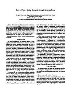
The simple network we simulated consists of nodes which are connected as a quadratic grid, like the one shown in Figure 2. Node 0 generates one packet each second and sends it to its neighbors. Whenever a node receives an unseen packet, it forwards it to all its neighbors. The connections between the nodes delay each packet by one second and drop the packets with a certain probability. Other aspects as collision or congestion were not considered, for which reason our simulation does not reflect a real computer network. Sender 0
1
2
3
4
5
6
7
9
10
11
13
14
15
8
Receiver 12
Fig. 2. The simple network used in the simulation for a size of 16 nodes We ran the simulation for network sizes ranging from 2 · 2 to 32 · 32 nodes with drop probabilities at each connection from 0 to 1. The node at the opposite corner of the sending node counts the packets it receives. We took the average delay and the total packet loss of the packets, traversing the network from one side to the other side, as qualitative measures. In order to compare the efficiency of the simulators, we measured the memory consumption and computation time. 10 seconds after the start Node 0 begins to send packets for 3600 seconds and the complete simulation is stopped after 5000 seconds simulation time. We implemented the simulation nearly identical in all four simulators. There is a class Network which contains the main-Method. It initializes the simulation and sets up the network. The class Packet represents a network packet and contains the id of the sender, the time it has been sent and an id which is unique for a specific sender. A class Node is responsible for representing the nodes of the network. It can generate packets, receive and forward packets and register whenever a packet has been received. Since the same packet can be received multiple times through different connections, all nodes maintain a linked list in which they store references to the packets they have seen. The longest time a 18
packet can stay in the network is when it is sent through every node and gets then back to the sender. It is therefore sufficient to keep only packets of the last (networksize + 1) seconds in this list. This cleaning-process takes place every 50 seconds. All nodes maintain a second list of connections they use. The class Connection stores to which node it is connected and can accept packets. Whenever a packet is accepted, it drops the packet with the given probability, delays the packet and delivers it to the node it is connected to. Sending a packet means to schedule an event in the appropriate Connection-class and receiving a packet means that the Connection-class schedules an event in the receiving node. The nodes use a class Stats which can count the number of packets being sent and received. This class prints out the accumulated data at the end of the simulation. Differences in the implementations have been only made if necessary, but we also tried to stick to the simulators paradigm. Since OMNeT++ supports events not directly, but has gates and connections to which a delay and biterror-rate4 can be assigned, we used the predefined connections instead of our own Connection-class. The network setup of the OMNeT++ implementation is also performed in a NED-file instead of a C++-Class. Another difference is that SimPy uses the process-oriented approach. The node-entities in the SimPysimulation use therefore a method which waits until a new packet is received, whereas the other three simulators provide an event-handler method for this. Since an entity in SimPy can have only one method which is running actively in a loop, we created separate entity classes for each node which are responsible for cleaning up the list of seen packets and generating Packets. 4.2
Examples of the Implementation
In order to outline the different concepts of the four simulators, we will now present in detail how the connections are implemented. As already mentioned we did not implement our own connection in OMNeT++. Figure 3 shows the part in the NED-file where the connections are created. It is part of the compound module which describes the whole network. Two nested for loops iterate through all nodes in the grid and for each node the connections to its neighbors are added. node[i].out++ --> error 0.5 delay 1 --> node[j].in++ means that a new output-gate of node i shall be connected to a new input gate of node j and that this connection has a bit-error-rate of 0.5 and a delay of 1 second. In our code variables conLoss and conDelay are used for the connection properties. These variables are set through the INI-file. There are four such lines in our source code, because a node in the grid is connected to its neighbor at each side. At the borders there are only two or three neighbors, for which reason we added an if-statement to each line which checks if the connection that shall be created is made to a valid neighbor. These few lines demonstrate also the drawback of using the NED-language: The node-id is computed in every line again and again, since one can not create variables at arbitrary positions in the 4
The drop probability we use in our own Connection-class is per packet, but if the length of the messages in OMNeT++ is set to 1 bit, this is the same.
19
code. In the if-condition of the latter two connections we had to use normal division together with the floor-function, since NED does not provide a divoperator for integers.
1 2 3
4
5
6
7
connections : for y = 0.. ySize -1 , x = 0.. xSize -1 do node [ x + y * xSize ]. out ++ --> error conLoss delay conDelay --> node [( x + y * xSize ) -1]. in ++ if ( x + y * xSize ) % xSize > 0; node [ x + y * xSize ]. out ++ --> error conLoss delay conDelay --> node [( x + y * xSize ) +1]. in ++ if ( x + y * xSize ) % xSize < xSize - 1; node [ x + y * xSize ]. out ++ --> error conLoss delay conDelay --> node [( x + y * xSize ) - xSize ]. in ++ if floor (( x + y * xSize ) / xSize ) > 0; node [ x + y * xSize ]. out ++ --> error conLoss delay conDelay --> node [( x + y * xSize ) + xSize ]. in ++ if floor (( x + y * xSize ) / xSize ) < ySize - 1; endfor ;
Fig. 3. A part of the network description in OMNeT++’s NED-language. Figure 4 shows a part of the Connection-class in the ns-3 implementation. This method send is called by nodes which want to send a packet through this connection. It gets the a smart-pointer of the Packet which shall be sent as parameter. At first a new random number is generated and if it is below the loss-threshold, the packet is dropped. Otherwise a new event is scheduled. This means in detail that after delay seconds the method receive of the object to is called with p as parameter.
1 2 3
void Connection :: send ( ns3 :: Ptr < Packet > p ) { if ( rand - > GetValue () < loss ) return ;
4
ns3 :: Simulator :: Schedule ( ns3 :: Seconds ( delay ) , & Node :: receive , to , p);
5
6
}
Fig. 4. The send-method in the connection-class of the ns-3 implementation. Figure 5 shows the corresponding part of the JiST implementation, which works basically in the same way. One difference is that invoking the event receive on the to object is done by simply calling this method. JiST itself translates this into the corresponding code for scheduling it as event. The second difference is that the time when this event shall be executed is not set explicit. Instead the time inside the send method is advanced before calling the event. The appropriate method in the SimPy implementation is shown in Figure 6. It works similar to the ones of the ns3 and the JiST implementation, but uses the process-based approach. It is called only once during start up and not every time a message is received. It therefore runs in an infinite loop. yield waitevent, self, self.event 20
1 2 3 4
void send ( Packet p ) { if ( rand . nextFloat () < loss ) { return ; }
5
JistAPI . sleep ( delay ) ;
6 7
to . receive ( p ) ;
8 9
}
Fig. 5. The send-method in the connection-class of the JiST implementation. means that the program shall wait until the object receives the event self.event. At next, the packet itself is extracted out of the signal parameter. Then a random number is generated and the packet is not processed any further if this random number is bigger than the threshold. yield hold, self, self.delay means to progress time of the object by self.delay seconds. After that happened, the received packet is sent to the receiving object self.to. This is done by calling the signal method of the event stored in self.to.event. Then the while-loop continues from its beginning and waits for the next packet.
1 2 3
def ACTIONS ( self ) : while 1: yield waitevent , self , self . event
4
packet = self . event . signalparam
5 6
if random () < self . loss : continue
7 8 9
yield hold , self , self . delay
10 11
self . to . event . signal ( packet )
12
Fig. 6. The Process Execution Method in the connection-class of the SimPy implementation.
4.3
Results
We used a computer with a 2.1 GHz AMD Dual-Core CPU and 2 GB of memory. Our simulations used only one CPU-core. We used OMNeT++ 3.4b2, ns-3.0.12, JiST/SWANS 1.0.6 with Sun Java 1.6.0 and SimPy-1.9.1 with Python 2.5. We ran the simulation for drop probabilities from 0 to 1 and network sizes from 4 to 1024. Figure 7 shows the average end-to-end packet delay depending on these values. The delay is rising with increasing network size, which is obvious since the packets have to pass more connections to reach the opposite corner. The 21
delay rises also slightly with increasing drop probability, because not all packets are able to take the shortest route. With a high drop probability and a large network size no packet at all makes its way through the network, leading to an infinite delay which is not plotted in this diagram. Figure 8 shows that the total packet loss is also rising slightly with increasing network size, since the drop probability is for each single connection and many connections have to be used in large networks. The packet loss is of course also rising with increasing drop probability.
OMNeT++ ns-3 JiST SimPy
90 80 70 60 50 40 Delay [s]30 20 10 0
1200 1000 1
0.8
800 0.6
Drop Probability
600 0.4
400 0.2
Network Size
200 0 0
Fig. 7. End-to-End Packet Delay
The retrieved data is nearly identical for all simulators, which proves the equivalence of the specific implementations. Slight derivations are normal since we used random data to decide if a packet is dropped or not. It is noteworthy that SimPy has a slightly higher packet loss for nearly all the values, which should not be the case. However we could not find any difference in the implementations which could cause this. We therefore suppose that this behavior can be attributed to the process-based simulation paradigm. Another possible explanation is a difference in the generation of random numbers. We ran the simulations by an external script which measures also the computation time and memory consumption of each simulation. The time includes everything from starting the simulation process until it finishes. The memory consumption is determined by reading /proc//status file of the Linux operating system. Before the simulation finishes, the simulation program prints out the packet delay, total loss and the content of this file. The external script parses the VmHWM field, which is the largest amount of memory ever owned by the process so far. Since the simulation has already ended, this is the memory peak value of the overall simulation. 22
OMNeT++ ns-3 JiST SimPy
1 0.8 0.6 Loss
0.4 0.2 0
1200 1000 1
0.8
800 0.6
Drop Probability
600 0.4
400 0.2
Network Size
200 0 0
Fig. 8. End-to-End Packet Loss Measuring the memory consumption of JiST is problematic since unneeded memory is not released directly, but at some unpredictable point in time by the Java garbage collector. Since this results in a much higher peak, the memory consumption of JiST is not comparable with the other simulators. We therefore did another measurement with a slightly modified version of our simulation where garbage collection is forced every time after some nodes have cleaned their lists of known packets. This dramatically decreases the maximum memory usage, but results in a slightly higher computation time. Both of these values thus have to be taken with care. Figure 9(a) and Figure 9(b) show the memory usage and computation time depending on the network size for a drop probability of 0.1 (run several times and averaged). It is not a surprise that memory consumption and computation time grow with increasing network size, because more data has to be stored and processed. One can also see that JiST with normal garbage collection needs more memory and a bit less computation time than the version with massive garbage collection (denoted by JiST-GC in the figures). Figure 9(c) and 9(d) show memory usage and computation time depending on the drop probability for a network size of 256 nodes (again for the average of several runs). Memory consumption and computation time both sink with an increasing drop probability. This is due to the fact that less packets make their way through the network if the drop probability is high and therefore less packets have to be stored and processed. One can see here again the difference between our two JiST-implementations. Regarding computation time one can say that SimPy performed very bad and it is in that point far behind the other three simulators. This may be in some parts due to implementation details, but is for sure because it uses the processoriented approach which requires time-demanding threading. JiST performed 23
200
8000 OMNeT++ ns-3 JiST SimPy JiST-GC
180
7000
OMNeT++ ns-3 JiST SimPy JiST-GC
160 6000
Computation Time [s]
Memory Usage [MB]
140 120 100 80
5000
4000
3000
60 2000 40 1000
20 0
0 0
200
400
600
800
1000
1200
0
200
400
600
Network Size
(a) Memory Usage
800
1000
1200
Network Size
(b) Computation Time
(drop probability = 0.1)
90
(drop probability = 0.1)
1000 OMNeT++ ns-3 JiST SimPy JiST-GC
80
OMNeT++ ns-3 JiST SimPy JiST-GC
900 800
70
700 Computation Time [s]
Memory Usage [MB]
60
50
40
600 500 400
30 300 20
200
10
100
0
0 0
0.2
0.4
0.6
0.8
1
0
Drop Probability
(c) Memory Usage
0.2
0.4
0.6
0.8
1
Drop Probability
(d) Computation Time
(drop probability = 0.1)
(network size = 256)
Fig. 9. Comparing simulator performance best regarding computation time and was especially for large network sizes better than ns-3 and OMNeT++. The memory usage of OMNeT++, ns-3 and SimPy is nearly equal. Our two JiST implementations however needed far more memory and especially the one with normal garbage collection performed worst. Simulations of wireless ad-hoc networks with ns-2 and JiST, which are presented in [9] and [3], showed that JiST used less memory than ns-2 and it is said that JiST/SWANS is very memory-efficient. Our results however show that JiST itself can also perform worse5 and that it might be only the network modules of SWANS which are more memory efficient than the ones of ns-2.
5
Conclusion
In this paper, we have surveyed recent developments in the area of network simulation toolkits. Looking closer at ns-3, OMNeT++, JiST/SWANS and SimPy, all four inspected simulators exhibit interesting concepts and projects as JiST show that also the fundamentals of discrete-event simulation can be implemented in a surprisingly different way. The comparison study we conducted reveals major differences in simulation performance and thus substantiates prior research results, such as [9]. 5
We have used ns-3 and not ns-2 for our simulation. Thus another reason might be that ns-3 is more memory efficient than ns-2.
24
Moreover, we emphasize that the results retrieved from the simulators were mostly equivalent, no matter what simulation tool was used. This is a straight consequence of the conformity of the simulation set-ups and models. We conclude that the conformity of network models and their parameter sets is important in order to achieve comparable and general results, and we hope that the discussion will shift from the choice of the right simulation tool more towards to the correct and reasonable design and use of simulation models.
Acknowledgments We would like to thank Andr´ as Varga for his helpful comments while writing this paper.
References 1. INET Framework for OMNeT++/OMNEST Documentation, 10 2006. http://www.omnetpp.org/doc/INET/neddoc/index.html [accessed on June, 2008]. 2. R. Barr. SWANS User Guide, 01 2006. http://jist.ece.cornell.edu/swans-user/index.html [accessed on June, 2008]. 3. R. Barr, Z. J. Haas, and R. van Renesse. Jist: an efficient approach to simulation using virtual machines: Research articles. Softw. Pract. Exper., 35(6):539–576, 2005. 4. C. D. Carothers, K. S. Perumalla, and R. M. Fujimoto. Efficient optimistic parallel simulations using reverse computation. ACM Transactions on Modeling and Computer Simulation (TOMACS, 9:224 – 253, 1999. 5. S. L. Ferenci, K. S. Perumalla, and R. M. Fujimoto. An approach for federating parallel simulators. In PADS ’00: Proceedings of the fourteenth workshop on Parallel and distributed simulation, pages 63–70, Washington, DC, USA, 2000. IEEE Computer Society. 6. Y. Gu, Y. Liu, and D. Towsley. On integrating fluid models with packet simulation. In INFOCOM 2004. Twenty-third AnnualJoint Conference of the IEEE Computer and Communications Societies, volume 4, pages 2856– 286, 2004. 7. T. R. Henderson, S. Roy, S. Floyd, and G. F. Riley. ns-3 project goals. In WNS2 ’06: Proceeding from the 2006 workshop on ns-2: the IP network simulator, page 13, New York, NY, USA, 2006. ACM. 8. D. Jefferson, B. Beckmann, and F. Wieland. Distributed simulation and the time warp operating system. In ACM Symposium on Operating Systems Principles, pages 77–93, 1987. 9. F. Kargl and E. Schoch. Simulation of manets: a qualitative comparison between jist/swans and ns-2. In MobiEval ’07: Proceedings of the 1st international workshop on System evaluation for mobile platforms, pages 41–46, New York, NY, USA, 2007. ACM. 10. G. Lencse and L. Muka. Combination and interworking of four modelling methods for infocommunications and business process systems. In Proceedings of the 2007 Industrial Simulation Conference (ISC’2007), 2007. 11. N. Matloff. Introduction to discrete-event simulation and the simpy language. http://heather.cs.ucdavis.edu/~matloff/156/ PLN/DESimIntro.pdf [accessed on May, 2008], Februrary 2008. 12. V. Naoumov and T. Gross. Simulation of large ad hoc networks. In MSWIM ’03: Proceedings of the 6th ACM international workshop on Modeling analysis and simulation of wireless and mobile systems, pages 50–57, New York, NY, USA, 2003. ACM. 13. G. F. Riley, T. M. Jaafar, R. M. Fujimoto, and M. H. Ammar. Space-parallel network simulations using ghosts. In Parallel and Distributed Simulation, 2004. PADS 2004. 18th Workshop, pages 170–177, 2004. 14. Y. A. Sekercioglu, A. Varga, and G. K. Egan. Parallel simulation made easy with omnet++. In Proceedings of the European Simulation Symposium (ESS 2003), 2003. 15. A. Varga and R. Hornig. An overview of the omnet++ simulation environment. In Simutools ’08, 2008.
25
16. A. Varga, Y. A. Sekercioglu, and G. K. Egan. A practical efficiency criterion for the null message algorithm. In Proceedings of the European Simulation Symposium (ESS 2003), 2003. 17. G. A. Vignaux and K. Muller. Simpy simplified, March 2008. http://simpy.sourceforge.net/SimPyDocs/ SManual.pdf [accessed on May, 2008]. 18. K. Walsh and E. G. Sirer. Staged simulation: A general technique for improving simulation scale and performance. ACM Trans. Model. Comput. Simul., 14(2):170–195, 2004.
26
Aachener Informatik-Berichte This list contains all technical reports published during the past five years. A complete list of reports dating back to 1987 is available from http://aib.informatik.rwth-aachen.de/. To obtain copies consult the above URL or send your request to: InformatikBibliothek, RWTH Aachen, Ahornstr. 55, 52056 Aachen, Email:
[email protected]
2003-01 2003-02
∗
2003-03 2003-04 2003-05 2003-06 2003-07
2003-08 2004-01 2004-02
∗
2004-03 2004-04 2004-05 2004-06 2004-07 2004-08 2004-09 2004-10 2005-01 2005-02
2005-03
∗
Jahresbericht 2002 J¨ urgen Giesl, Ren´e Thiemann: Size-Change Termination for Term Rewriting J¨ urgen Giesl, Deepak Kapur: Deciding Inductive Validity of Equations J¨ urgen Giesl, Ren´e Thiemann, Peter Schneider-Kamp, Stephan Falke: Improving Dependency Pairs Christof L¨ oding, Philipp Rohde: Solving the Sabotage Game is PSPACEhard Franz Josef Och: Statistical Machine Translation: From Single-Word Models to Alignment Templates Horst Lichter, Thomas von der Maßen, Alexander Nyßen, Thomas Weiler: Vergleich von Ans¨ atzen zur Feature Modellierung bei der Softwareproduktlinienentwicklung J¨ urgen Giesl, Ren´e Thiemann, Peter Schneider-Kamp, Stephan Falke: Mechanizing Dependency Pairs Fachgruppe Informatik: Jahresbericht 2003 Benedikt Bollig, Martin Leucker: Message-Passing Automata are expressively equivalent to EMSO logic Delia Kesner, Femke van Raamsdonk, Joe Wells (eds.): HOR 2004 – 2nd International Workshop on Higher-Order Rewriting Slim Abdennadher, Christophe Ringeissen (eds.): RULE 04 – Fifth International Workshop on Rule-Based Programming Herbert Kuchen (ed.): WFLP 04 – 13th International Workshop on Functional and (Constraint) Logic Programming Sergio Antoy, Yoshihito Toyama (eds.): WRS 04 – 4th International Workshop on Reduction Strategies in Rewriting and Programming Michael Codish, Aart Middeldorp (eds.): WST 04 – 7th International Workshop on Termination Klaus Indermark, Thomas Noll: Algebraic Correctness Proofs for Compiling Recursive Function Definitions with Strictness Information Joachim Kneis, Daniel M¨ olle, Stefan Richter, Peter Rossmanith: Parameterized Power Domination Complexity Zinaida Benenson, Felix C. G¨artner, Dogan Kesdogan: Secure MultiParty Computation with Security Modules Fachgruppe Informatik: Jahresbericht 2004 Maximillian Dornseif, Felix C. G¨artner, Thorsten Holz, Martin Mink: An Offensive Approach to Teaching Information Security: “Aachen Summer School Applied IT Security” J¨ urgen Giesl, Ren´e Thiemann, Peter Schneider-Kamp: Proving and Disproving Termination of Higher-Order Functions
27
2005-04 2005-05 2005-06 2005-07
2005-08 2005-09 2005-10 2005-11 2005-12
2005-13 2005-14 2005-15 2005-16 2005-17 2005-18
2005-19 2005-20
2005-21 2005-22 2005-23 2005-24 2006-01 2006-02
∗
Daniel M¨ olle, Stefan Richter, Peter Rossmanith: A Faster Algorithm for the Steiner Tree Problem Fabien Pouget, Thorsten Holz: A Pointillist Approach for Comparing Honeypots Simon Fischer, Berthold V¨ ocking: Adaptive Routing with Stale Information Felix C. Freiling, Thorsten Holz, Georg Wicherski: Botnet Tracking: Exploring a Root-Cause Methodology to Prevent Distributed Denial-ofService Attacks Joachim Kneis, Peter Rossmanith: A New Satisfiability Algorithm With Applications To Max-Cut Klaus Kursawe, Felix C. Freiling: Byzantine Fault Tolerance on General Hybrid Adversary Structures Benedikt Bollig: Automata and Logics for Message Sequence Charts Simon Fischer, Berthold V¨ ocking: A Counterexample to the Fully Mixed Nash Equilibrium Conjecture Neeraj Mittal, Felix Freiling, S. Venkatesan, Lucia Draque Penso: Efficient Reductions for Wait-Free Termination Detection in Faulty Distributed Systems Carole Delporte-Gallet, Hugues Fauconnier, Felix C. Freiling: Revisiting Failure Detection and Consensus in Omission Failure Environments Felix C. Freiling, Sukumar Ghosh: Code Stabilization Uwe Naumann: The Complexity of Derivative Computation Uwe Naumann: Syntax-Directed Derivative Code (Part I: TangentLinear Code) Uwe Naumann: Syntax-directed Derivative Code (Part II: Intraprocedural Adjoint Code) Thomas von der Maßen, Klaus M¨ uller, John MacGregor, Eva Geisberger, J¨org D¨orr, Frank Houdek, Harbhajan Singh, Holger Wußmann, Hans-Veit Bacher, Barbara Paech: Einsatz von Features im SoftwareEntwicklungsprozess - Abschlußbericht des GI-Arbeitskreises “Features” Uwe Naumann, Andre Vehreschild: Tangent-Linear Code by Augmented LL-Parsers Felix C. Freiling, Martin Mink: Bericht u ¨ ber den Workshop zur Ausbildung im Bereich IT-Sicherheit Hochschulausbildung, berufliche Weiterbildung, Zertifizierung von Ausbildungsangeboten am 11. und 12. August 2005 in K¨oln organisiert von RWTH Aachen in Kooperation mit BITKOM, BSI, DLR und Gesellschaft fuer Informatik (GI) e.V. Thomas Noll, Stefan Rieger: Optimization of Straight-Line Code Revisited Felix Freiling, Maurice Herlihy, Lucia Draque Penso: Optimal Randomized Fair Exchange with Secret Shared Coins Heiner Ackermann, Alantha Newman, Heiko R¨ oglin, Berthold V¨ ocking: Decision Making Based on Approximate and Smoothed Pareto Curves Alexander Becher, Zinaida Benenson, Maximillian Dornseif: Tampering with Motes: Real-World Physical Attacks on Wireless Sensor Networks Fachgruppe Informatik: Jahresbericht 2005 Michael Weber: Parallel Algorithms for Verification of Large Systems
28
2006-03 2006-04 2006-05
2006-06 2006-07 2006-08 2006-09 2006-10
2006-11 2006-12
2006-13 2006-14
2006-15 2006-16 2006-17 2007-01 2007-02
2007-03 2007-04 2007-05 2007-06
∗
Michael Maier, Uwe Naumann: Intraprocedural Adjoint Code Generated by the Differentiation-Enabled NAGWare Fortran Compiler Ebadollah Varnik, Uwe Naumann, Andrew Lyons: Toward Low Static Memory Jacobian Accumulation Uwe Naumann, Jean Utke, Patrick Heimbach, Chris Hill, Derya Ozyurt, Carl Wunsch, Mike Fagan, Nathan Tallent, Michelle Strout: Adjoint Code by Source Transformation with OpenAD/F Joachim Kneis, Daniel M¨ olle, Stefan Richter, Peter Rossmanith: Divideand-Color Thomas Colcombet, Christof L¨ oding: Transforming structures by set interpretations Uwe Naumann, Yuxiao Hu: Optimal Vertex Elimination in SingleExpression-Use Graphs Tingting Han, Joost-Pieter Katoen: Counterexamples in Probabilistic Model Checking Mesut G¨ unes, Alexander Zimmermann, Martin Wenig, Jan Ritzerfeld, Ulrich Meis: From Simulations to Testbeds - Architecture of the Hybrid MCG-Mesh Testbed Bastian Schlich, Michael Rohrbach, Michael Weber, Stefan Kowalewski: Model Checking Software for Microcontrollers Benedikt Bollig, Joost-Pieter Katoen, Carsten Kern, Martin Leucker: Replaying Play in and Play out: Synthesis of Design Models from Scenarios by Learning Wong Karianto, Christof L¨ oding: Unranked Tree Automata with Sibling Equalities and Disequalities Danilo Beuche, Andreas Birk, Heinrich Dreier, Andreas Fleischmann, Heidi Galle, Gerald Heller, Dirk Janzen, Isabel John, Ramin Tavakoli Kolagari, Thomas von der Maßen, Andreas Wolfram: Report of the GI Work Group “Requirements Management Tools for Product Line Engineering” Sebastian Ullrich, Jakob T. Valvoda, Torsten Kuhlen: Utilizing optical sensors from mice for new input devices Rafael Ballagas, Jan Borchers: Selexels: a Conceptual Framework for Pointing Devices with Low Expressiveness Eric Lee, Henning Kiel, Jan Borchers: Scrolling Through Time: Improving Interfaces for Searching and Navigating Continuous Audio Timelines Fachgruppe Informatik: Jahresbericht 2006 Carsten Fuhs, J¨ urgen Giesl, Aart Middeldorp, Peter Schneider-Kamp, Ren´e Thiemann, and Harald Zankl: SAT Solving for Termination Analysis with Polynomial Interpretations J¨ urgen Giesl, Ren´e Thiemann, Stephan Swiderski, and Peter SchneiderKamp: Proving Termination by Bounded Increase Jan Buchholz, Eric Lee, Jonathan Klein, and Jan Borchers: coJIVE: A System to Support Collaborative Jazz Improvisation Uwe Naumann: On Optimal DAG Reversal Joost-Pieter Katoen, Thomas Noll, and Stefan Rieger: Verifying Concurrent List-Manipulating Programs by LTL Model Checking
29
2007-07 2007-08 2007-09
2007-10 2007-11 2007-12 2007-13
2007-14
2007-15 2007-16
2007-17 2007-18 2007-19 2007-20 2007-21
2007-22 2008-01 2008-02 2008-03 2008-04 2008-05 2008-06
2008-08 2008-09
∗
Alexander Nyßen, Horst Lichter: MeDUSA - MethoD for UML2-based Design of Embedded Software Applications Falk Salewski and Stefan Kowalewski: Achieving Highly Reliable Embedded Software: An empirical evaluation of different approaches Tina Kraußer, Heiko Mantel, and Henning Sudbrock: A Probabilistic Justification of the Combining Calculus under the Uniform Scheduler Assumption Martin Neuh¨ außer, Joost-Pieter Katoen: Bisimulation and Logical Preservation for Continuous-Time Markov Decision Processes Klaus Wehrle (editor): 6. Fachgespr¨ ach Sensornetzwerke Uwe Naumann: An L-Attributed Grammar for Adjoint Code Uwe Naumann, Michael Maier, Jan Riehme, and Bruce Christianson: Second-Order Adjoints by Source Code Manipulation of Numerical Programs Jean Utke, Uwe Naumann, Mike Fagan, Nathan Tallent, Michelle Strout, Patrick Heimbach, Chris Hill, and Carl Wunsch: OpenAD/F: A Modular, Open-Source Tool for Automatic Differentiation of Fortran Codes Volker Stolz: Temporal assertions for sequential and concurrent programs Sadeq Ali Makram, Mesut G¨ une¸c, Martin Wenig, Alexander Zimmermann: Adaptive Channel Assignment to Support QoS and Load Balancing for Wireless Mesh Networks Ren´e Thiemann: The DP Framework for Proving Termination of Term Rewriting Uwe Naumann: Call Tree Reversal is NP-Complete Jan Riehme, Andrea Walther, J¨org Stiller, Uwe Naumann: Adjoints for Time-Dependent Optimal Control Joost-Pieter Katoen, Daniel Klink, Martin Leucker, and Verena Wolf: Three-Valued Abstraction for Probabilistic Systems Tingting Han, Joost-Pieter Katoen, and Alexandru Mereacre: Compositional Modeling and Minimization of Time-Inhomogeneous Markov Chains Heiner Ackermann, Paul W. Goldberg, Vahab S. Mirrokni, Heiko R¨ oglin, and Berthold V¨ ocking: Uncoordinated Two-Sided Markets Fachgruppe Informatik: Jahresbericht 2007 Henrik Bohnenkamp, Marielle Stoelinga: Quantitative Testing Carsten Fuhs, J¨ urgen Giesl, Aart Middeldorp, Peter Schneider-Kamp, Ren´e :Thiemann, Harald Zankl: Maximal Termination Uwe Naumann, Jan Riehme: Sensitivity Analysis in Sisyphe with the AD-Enabled NAGWare Fortran Compiler Frank G. Radmacher: An Automata Theoretic Approach to the Theory of Rational Tree Relations Uwe Naumann, Laurent Hascoet, Chris Hill, Paul Hovland, Jan Riehme, Jean Utke: A Framework for Proving Correctness of Adjoint Message Passing Programs George B. Mertzios, Stavros D. Nikolopoulos: The λ-cluster Problem on Parameterized Interval Graphs George B. Mertzios, Walter Unger: An optimal algorithm for the k-fixedendpoint path cover on proper interval graphs
30
2008-10 2008-11 2008-12 2008-13
2008-14 2008-15
∗
George B. Mertzios, Walter Unger: Preemptive Scheduling of EqualLength Jobs in Polynomial Time George B. Mertzios: Fast Convergence of Routing Games with Splittable Flows Joost-Pieter Katoen, Daniel Klink, Martin Leucker, Verena Wolf: Abstraction for stochastic systems by Erlang’s method of stages Beatriz Alarc´ on, Fabian Emmes, Carsten Fuhs, J¨ urgen Giesl, Ra´ ul Gutierrez, Salvador Lucas, Peter Schneider-Kamp, Ren´e Thiemann: Improving Context-Sensitive Dependency Pairs Bastian Schlich: Model Checking Software for Microcontrollers Joachim Kneis, Alexander Langer, Peter Rossmanith: A New Algorithm for Finding Trees with Many Leaves
These reports are only available as a printed version.
Please contact
[email protected] to obtain copies.
31