A dual version that computes convex hulls was discovered by Chand and Kapur[2], and ...... Robert, and P. Yamamoto, âOrthogonal Weighted Linear L1.
A Pivoting Algorithm for Convex Hulls and Vertex Enumeration of Arrangements and Polyhedra David Avis School of Computer Science McGill University 3480 University, Montreal, Quebec H3A 2A7 Komei Fukuda Graduate School of Systems Management The University of Tsukuba Otsuka, Bunkyo-ku, Tokyo 112 Research Report B-237 Tokyo Institute of Technology, Dept. of Information Science November 1990
ABSTRACT We present a new pivot-based algorithm which can be used with minor modification for the enumeration of the facets of the convex hull of a set of points, or for the enumeration of the vertices of an arrangement or of a convex polyhedron, in arbitrary dimension. The algorithm has the following properties: (a) No additional storage is required beyond the input data; (b) The output list produced is free of duplicates; (c) The algorithm is extremely simple, requires no data structures, and handles all degenerate cases; (d) The running time is output sensitive for non-degenerate inputs; (e) The algorithm is easy to efficiently parallelize. For example, the algorithm finds the v vertices of a polyhedron in R d defined by a nondegenerate system of n inequalities (or dually, the v facets of the convex hull of n points in R d , where each facet contains exactly d given points) in time O(ndv) and O(nd) space. The v vertices in a simple arrangement of n hyperplanes in R d can be found in O(n2 dv) time and O(nd) space complexity. The algorithm is based on inverting finite pivot algorithms for linear programming.
-21. Introduction In this paper we give an algorithm, which with minor variations can be used to solve three basic enumeration problems in computational geometry: facets of the convex hull of a set of points, vertices of a convex polyhedron given by a system of linear inequalities, and vertices of an arrangement of hyperplanes. The algorithm is based on pivoting and has many nice properties. Among these are that no additional space is required apart from that required to store the input, and that the algorithm produces a list that is free of duplicates even for degenerate inputs. The algorithm is based on "inverting" finite pivoting algorithms for linear programming. No special knowledge of linear programming or arrangements is assumed, and necessary terminology is defined here. For additional information the reader is referred to Chva´tal[3] for linear programming and Edelsbrunner[6] for arrangements. In the the rest of this section we give an informal description of the algorithm beginning with the vertex enumeration problem for convex polyhedra. Suppose we have a system of linear inequalities defining a polyhedron in R d and a vertex of that polyhedron. A vertex is specified by giving the indices of d inequalities whose bounding hyperplanes intersect at the vertex. For any given linear objective function, the simplex method generates a path along edges of the polyhedron until a vertex maximizing this objective function is found. For simplicity, let us assume for the moment that the optimum vertex is contained on exactly d bounding hyperplanes. The path is found by pivoting, which involves interchanging one of the equations defining the vertex with one not currently used. The path chosen from an initial given vertex depends on the pivot rule used. In fact, care must be taken because some pivot rules generate cycles and do not lead to the optimum vertex. However, a particularly simple rule, known as Bland’s rule or the least subscript rule[1], guarantees a unique path from any starting vertex to the optimum vertex. If we look at the set of all such paths from all vertices of the polyhedron, we get a spanning tree of the edge graph of the polyhedron rooted at the optimum vertex. Our algorithm simply starts at an "optimum vertex" and traces out the tree in depth first order by "reversing" Bland’s rule. A remarkable feature is that no additional storage is needed at intermediate nodes in the tree. Going down the tree we explore all valid "reverse" pivots in lexicographical order from any given intermediate node. Going back up the tree, we simply use Bland’s rule to return us to the parent node along with the current pivot indices. From there it is simple to continue by considering the next lexicographic "reverse" pivot, etc. The algorithm is therefore non-recursive and requires no stack or other data structure. One possible difficulty arises at so-called degenerate vertices, vertices which lie on more than d bounding hyperplanes. It is desirable to report each vertex once only, and this can be achieved without storing the output and searching. By using duality, we can also use this algorithm for enumerating the facets of the convex hull of a set of points in R d . It can also be used for enumerating all of the vertices of the Voronoi Diagram of a set of points in R d , since this can be reformulated as a convex hull problem in R d+1 (see [6] ). A variant of this method can be used for vertex enumeration of arrangements. Again consider the linear programming problem discussed above. Each inequality defining the polyhedron is bounded by a hyperplane. The corresponding arrangement of hyperplanes contains many vertices, some of which are vertices of the polyhedron, known as feasible vertices. The others are known as infeasible vertices. A recent development in linear programming is a pivot rule that starts at any vertex of this arrangement, feasible or infeasible, and finds a unique path to the optimum solution of the linear program. This is known as the criss-cross method, and was developed independently by Terlaky[15], [16] and Wang[18]. Reversing this algorithm along the lines described above yields our algorithm for enumerating vertices of arrangements. The problems discussed in this paper have a long history, which we briefly mention here. The problem of enumerating all of the vertices of a polyhedron is surveyed by Mattheiss and Rubin in[11] and by Dyer in[4]. There are essentially two classes of methods. One class is based on pivoting and is discussed in detail in[4] and[3]. In this method a depth first search is initiated from a vertex by trying all possible simplex pivots. The difficulty is in determining whether or not a vertex has already been visited. For this
-3all vertices must be stored in a balanced AVL-tree. An implementation that takes O(nd 2 v) time and O(dv) space for a polyhedron with v vertices defined by a non-degenerate system of n inequalities in R d is given in[4]. A dual version that computes convex hulls was discovered by Chand and Kapur[2], and has similar complexity. Using sophisticated data structures, Seidel[13] was able to achieve a running time of O(d 3 v log n + nf (d − 1, n − 1)) for sets of n points in R d , when each facet contains exactly d given points. Here f (d, n) is the time to solve a linear program with n constraints in d variables, and v is the number of facets of the convex hull. The space required for this algorithm is O(nd/2 ). The algorithm presented in this paper fits into this class. It achieves O(dvn) time and O(dn) space complexity for facet enumeration of the convex hull of n points in R d , when each facet contains exactly d given points. To the authors’ knowledge, it is the only algorithm known that has non-exponential space requirements in the worst case. A second class of methods for computing the vertices of a convex polyhedron is the "double description" method of Motzkin et al.[12] that dates back to 1953. In fact the origin of these methods is even earlier, as the double description method is in fact dual to the Fourier-Motzkin method for the solution of linear inequality systems. In the double description method, the polyhedron is constructed sequentially by adding a constraint at a time. All new vertices produced must lie on the hyperplane bounding the constraint currently being inserted. A dual version for constructing convex hulls is known as the "beneath and beyond" method. Assuming the dimension d is fixed, the fastest algorithm of this class again uses sophisticated data structures and is due to Seidel [14] (also see [6] ). It takes O(nd/2+1 ) time and O(nd/2 ) space. With d fixed, the complete facial structure of a hyperplane arrangement can be constructed by an algorithm due to Edelsbrunner, O’Rourke and Seidel [5] in optimal time and space O(n d ). The algorithm works by inserting the hyperplanes one at a time and can handle degenerate cases. Again with d fixed, a method for enumerating just the edges and vertices (with repetitions) in O(n d ) time and O(n) space is given by Edelsbrunner et al.[7]. Houle et al.[10] give several applications in data approximation where it is required to enumerate all vertices of an arrangement. In the next section we begin by introducing the notion of a dictionary for a system of equations. Next we show how the problems mentioned in the title can be transformed into the enumeration of certain types of dictionaries. In the third section we give the algorithm for enumeration of dictionaries. Finally in the last section we discuss complexity issues, and other properties of the algorithm proposed. 2. Dictionaries Let A be a m×n matrix, with columns indexed by the set E = {1, 2, . . . , n}. Fix distinct indices f and g of E. Consider the system of equations: A x = 0, x g = 1.
(2.1)
For any J ⊆ E, x J denotes the subvector of x indexed by J, and A J denotes the submatrix of A consisting of columns indexed by J. A basis B for (2.1) is a subset of E of cardinality m containing f but not g, for which A B is nonsingular. We will only be concerned with systems (2.1) that have at least one basis, and will assume this for the rest of the paper. Given any basis B, we can transform (2.1) into the dictionary: x B = − A−1 B AN x N = A x N ,
(2.2)
where N = E − B is the co − basis, and A denotes − A−1 B A N . A is called the coefficient matrix of the dictionary, with rows indexed by B and columns indexed by N , so that A = (aij : i ∈B, j ∈N ). Note that the co-basis always contains the index g.
-4A variable x i is primal feasible if i ∈B − f and aig ≥ 0. A variable x j is dual feasible if j ∈N − g and a fj ≤ 0. A dictionary is primal feasible if x i is primal feasible for all i ∈B − f and dual feasible if x j is dual feasible for all j ∈N − g. A dictionary is optimal if it is both primal and dual feasible. An optimal dictionary is shown schematically in Figure 2.1. g f
B− f
N−g O - O - O - O - O - O -
O + O + O + O + O +
= A
Figure 2.1 : An Optimal Dictionary ( O + = non-negative entry, O − = non-positive entry ) A basic solution to (2.1) is obtained from a dictionary by setting x N −g = 0, x g = 1. If any basic variable has value zero, we call the basic solution and corresponding dictionary degenerate. In section 2 of the paper we give an algorithm for enumerating all distinct basic solutions of the system (2.1) without repetition, using only the space required to store the input. The algorithm is initiated with an optimal dictionary. A variant of the algorithm enumerates all primal feasible dictionaries reporting the corresponding basic feasible solutions without repetition. In the following subsections, we show how the problems mentioned in the title can be transformed into the problem of enumerating basic (feasible) solutions of a system of equations in the form (2.1). 2.1. Vertex enumeration in hyperplane arrangements A hyperplane in R d , d ≥ 0, is denoted by the pair (b, c), where b is a vector of length d and c is a scalar, and is the solution set of the equation by = c, y = (y j : j = 1, . . . , d). A hyperplane arrangement is a collection of n0 hyperplanes (bi , c i ), for some integer n0 . A vertex of the arrangement is the unique solution to the system of d equations corresponding to d intersecting hyperplanes. The vertex enumeration problem for hyperplane arrangements is to list all of the vertices of an arrangement. It is a simple matter to find a vertex of an arrangement, or show that none exists, since vertices correspond to subsets of d hyperplanes whose normal vectors bi are linearly independent. We only consider arrangements that contain at least one vertex. We may assume by relabeling if necessary that the vectors {b n0 −d+1 , . . . , b n0 } are linearly independent. Consider the system of equations x i = c i x n0 +1 − bi y,
i = 1, . . . , n0 .
By assumption, the last d equations are linearly independent, and so the variables y 1 , . . . , y d can be expressed in terms of x n0 −d+1 , . . . , x n0 , and eliminated from the first n0 − d equations. This results in a system of the form: x B = Ax N , for a suitable (n0 − d) ×(d + 1) matrix A, where B = {1, . . . , n0 − d} and N = {n0 − d + 1, . . . , n0 + 1}. Furthermore, by a change of variables if necessary, we may assume that each ai,n0 +1 is non-negative. We augment A by adding a row of of all -1 ’s. We augment B by adding index n0 + 2. Setting
-5f = n0 + 2, g = n0 + 1, m = n0 − d + 1, n = n0 + 2, we have constructed an optimal dictionary. This dictionary is obtained from the following system which has the form of (2.1): Ix B − Ax N = 0,
x g = 1.
(2.3)
It is easy to show that for every co-basis N of (2.3), the set of d hyperplanes indexed by N − g intersect at some vertex of the arrangement. The vertex can be computed by setting x i = aig i ∈B − f , x j = 0
j ∈N − g
and solving for y , which was expressed in terms of x n0 −d+1 , . . . , x n0 . Similarly every index set of d intersecting hyperplanes augmented by index f gives a co-basis for (2.3). We say that a vertex is degenerate if it is contained in more than d hyperplanes. For such vertices, there may be many corresponding bases of (2.3), each giving rise to a degenerate dictionary. An essential part of our enumeration algorithm will be to only output a degenerate vertex once. 2.2. Vertex enumeration for Polyhedra A (convex) polyhedron P is the solution set to a system of n0 inequalities in d non-negative variables: P = {y ∈R d | A′y ≤ b, y ≥ 0},
(2.4)
where A′ is an n0 × d matrix and b is a n0 -vector. A vertex of the polyhedron is a vector y ∈P that satisfies a linearly independent set of d of the inequalities as equations. The vertex enumeration problem for P is to enumerate all of its vertices. In fact to find even a single vertex of P is computationally equivalent to linear programming. As we wish to separate this from the enumeration problem, we will assume we are given an initial vertex. By transforming the problem as necessary, we may assume that the origin is the given vertex. This implies that the vector b is non-negative. We also note that the assumption of nonnegative variables is not essential: a system of inequalities in unrestricted variables with known feasible point can be transformed into a system such as (2.4) along the lines described in the previous subsection. Let n = n0 + d + 2, f = n − 1, g = n, B = {1, . . . , n0 , n − 1} and N = {n0 + 1, . . . , n0 + d, n}. Consider the following system of equations in the form of (2.1): 1x N −g + x f Ix B− f + A′x N −g
=0
− bx g = 0
(2.5)
x g = 1. Here I is an identity matrix and 1 is a vector of all ones, of appropriate dimensions. Set m = n0 + 1 and let A be the m×n matrix corresponding to the coefficients in the first m equations of (2.5). Then (2.2) is an optimal dictionary for the system (2.5). It can be shown that each primal feasible dictionary for (2.5) has a basic solution which gives a vertex y of P: set y j = x n0 + j , j = 1, . . . , d. A vertex of P is degenerate if it satisfies more than d inequalities of (2.4) as equations. Again, degenerate vertices correspond to degenerate dictionaries. In order to enumerate all vertices of P, it is sufficient to enumerate all primal feasible dictionaries for (2.5), outputting a degenerate basic solution once only.
-62.3. Facet enumeration of the convex hull of a set of points Let Q = {q 1 , . . . , q n0 } denote a set of n0 points in R d . A facet of the convex hull of Q is a hyperplane containing d affinely independent points of Q. There is no loss of generality in assuming that the origin is contained in the convex hull of Q. By employing a standard duality between points and hyperplanes, we may transform this problem into a vertex enumeration problem for a convex polyhedron. 3. Enumeration of Dictionaries Suppose we are given a system of equations of the form (2.1), for some m×n matrix A. The linear programming problem (LP) for (2.1) is to maximize x f over (2.1) subject to the additional constraint that each variable except x f and x g is non-negative. Each optimal dictionary is a solution to LP. To begin with, we will assume that there is a unique optimal dictionary. A pivot (r, s) on a basis B, and corresponding dictionary x B = Ax B , is an interchange of some r ∈B − f with some index s ∈N − g giving a new basis B′. The new coefficient matrix A′ = (a′ij ) is given by a′rs = −
arj ais arj a 1 , a′is = is , a′rj = , a′ij = aij − , ars ars ars ars
( i ∈B − r, j ∈N − s ).
(3.1)
The pivot is primal feasible (respectively, dual feasible) if both of the dictionaries corresponding to B and B′ are primal (respectively, dual) feasible. The simplex method is a method of solving LP by beginning with an initial dictionary and pivoting until an optimal dictionary is found. We consider two rules for choosing a pivot. The first rule, known as Bland’s rule, performs primal feasible pivots. Let B be a basis such that the dictionary (2.2) is primal feasible. Bland’s Rule. (1)
Let s be the smallest index such that x s is dual infeasible, that is, a fs > 0. aig : i ∈B − f , ais < 0}. Let r be the smallest index obtaining this minimum. (2) Set λ = min { − ais The pivot (r, s) maintains the primal feasibility of the dictionary. If step (1) does not apply, the dictionary is also dual feasible and hence optimal. The second rule, known as the criss-cross rule, starts with any basis. Criss-Cross Rule (1)
Let i ≠ f , g be the smallest index such that x i is (primal or dual)infeasible.
(2)
If i ∈B, let r = i and let s be the minimum index such that ars > 0, otherwise let s = i and let r be the minimum index such that ars < 0.
The criss-cross pivot (r, s) interchanges x r and x s , and may not preserve either primal or dual feasibility. If step (1) does not apply then the dictionary is optimal. The validity of these rules is given by the following proposition. Part (a) is proved in[1] and part (b) in[15] for linear programs, and in[16] [18] in the more general setting of oriented matroids. A simple proof of part (b) also appears in [9]. Proposition 3.1. Let (2.1) be a system that admits an optimal dictionary and let B be any basis. (a) If B is primal feasible, then successive application of Bland’s rule leads to an optimal dictionary, and each basis generated is primal feasible. (b) Successive application of the criss-cross rule starting with basis B leads to an optimal dictionary.
-73.1. Unique Optimal Dictionaries In this subsection we give a dictionary enumeration algorithm for systems (2.1) that admit a unique optimal dictionary. Consider a graph where vertices are dictionaries and two vertices are adjacent if the corresponding two dictionaries differ in only one basic variable. Then part (b) of the proposition tells us that there is a unique path consisting of criss-cross pivots from any dictionary to the optimal dictionary. The set of all such paths gives us a spanning tree in this graph. Consider a non-optimal dictionary D with basis B. Let (r, s), r ∈B − f , s ∈N − g, be the pivot obtained by applying the criss-cross rule to D giving a dictionary D′. We call (s, r) a reverse criss − cross pivot for D′. Suppose we start at the optimal dictionary and explore reverse criss-cross pivots in lexicographic order. This corresponds to a depth first search of the spanning tree defined above. When moving down the tree, each dictionary is encountered exactly once. A similar analysis applies to part (a) of the proposition. We form a similar graph, except that vertices are just the primal feasible dictionaries. We define a reverse Bland pivot in the analogous way. A depth first search of this graph provides all primal feasible dictionaries. Our enumeration algorithm search for dictionaries is given in Figure 3.1. For a given system (2.1) we have an initial basis B = {1, . . . , m}, co-basis N = {m + 1, . . . , n} and optimal dictionary x B = Ax N . We further assume that f = 1, g = n, and that m and n are global constants. The efficiency of the procedure depends greatly on the procedure reverse. The simplest way to check if (r, s), r ∈B − f , s ∈N − g, is a reverse pivot is to actually perform the pivot, then use procedure select − pivot on the new dictionary. If this produces the same pair of variables, then (r, s) is a valid reverse pivot. Since a pivot involves O(mn) operations, a faster method is desirable. In fact to determine the pivot by the criss-cross or Bland’s rules, the entire dictionary is not required by procedure select − pivot. To test whether A arises from a coefficient matrix A′ by a criss-cross (resp., Bland ) pivot interchanging B[i] with N [ j], it is only necessary to examine rows f , i and columns j, g of A′. These can be computed from A in O(m + n) time, and checked to see if (B[i], N [ j]) is a criss-cross (resp., Bland) pivot. Further savings are possible, as certain potential reverse pivots can be eliminated without any pivoting. For the criss-cross rule we have the following necessary condition for a reverse pivot. Proposition 3.2 If (s, r), s ∈B − f and r ∈N − g, is a valid reverse criss-cross pivot for a dictionary x B = Ax N , then either (a)
a sg > 0, a sr > 0, a sj ≥ 0 for j ∈N − g, j < s, or
(b)
a fr < 0, a sr < 0, air ≤ 0 for i ∈B − f , i < r.
Proof: Let A′ = (a′ij ), with basis B′ and co-basis N ′, be a dictionary that yields A after the valid cross pivot (r, s), with r ∈B′ − f , and s ∈N ′ − g. One of the indices r, s must be the smallest infeasible index in A′. Suppose first that it is r. By the criss-cross rule we must therefore have a′rg < 0, a′rs > 0, and a′rj ≤ 0 for all j ∈N ′ − g, j < s. Now applying the pivot formula (3.1) to the pivot row of A′ we obtain the signs indicated in part (a) of the proposition in A. A similar analysis applies to the case where s is the smallest infeasible index in A′, giving the sign pattern of part (b) of the proposition. For reversing Bland’s rule, we can exploit the fact that the reverse pivot must maintain primal feasibility. aig : i ∈B − f , air < 0}. air If (s, r), s ∈B − f , is a valid reverse Bland’s rule pivot then s must be an index that obtains this minimum.
Proposition 3.3 Let x B = Ax N be a dictionary, let r ∈N − g and set λ = min { −
Proof: Under the conditions of the proposition, if s is not an index realizing the minimum, then the dictionary obtained after the pivot (s, r) is not primal feasible. In the next section, we see how this simple observation reduces the complexity of search in non-degenerate situations. The procedure lex − min is used to ensure that each basic solution is output exactly once, when the lexicographically minimum basis for that basic solution is reached. The correctness of the procedure is
-8-
________________________________________________________________________________ procedure search (B, N , A); /* B = {1, . . . , m}, N = {m + 1, . . . , n}, f = 1, g = n, x B = Ax N is a unique optimal dictionary for a system (2.1) */ begin i: = 2; j: = 1; repeat while ( i ≤ m and not reverse (B, N , A, i, j) ) increment (i, j); if ( i ≤ m ) then /* reverse pivot found */ begin pivot (B, N , A, i, j); if lex-min (B, N , A) then print (B); i: = 2; j: = 1; end; else /* go back to previous dictionary */ begin select-pivot ( A, i, j); pivot (B, N , A, i, j); increment (i, j); end; until (i > m and B[m] = m ) end; /* search */ function reverse (B, N , A, i, j):boolean; /* true if (s, r), with s = B[i], r = N [ j], is a valid reverse cross-pivot (resp., Bland-pivot ) for A, otherwise false */ procedure pivot (B, N , A, i, j); /* pivot A on row i and column j, update B and N . Reorder as necessary and set i and j to be the indices of the interchanged B[i] and N [ j]. */ function lex-min (B, N , A):boolean; /* true if A is non-degenerate, or degenerate and B is the lexicographically minimum basis for this basic solution, else false */ procedure select-pivot ( A, i, j); /* Find criss-cross (resp., Bland) pivot for coefficient matrix A. Return the index i of the pivot row and index j of the pivot column*/ procedure increment (i, j); begin j: = j + 1; if ( j = n − m) then begin j: = 1; i: = i + 1; end; end; /* increment */ Figure 3.1 ________________________________________________________________________________
-9based on the following proposition. Proposition 3.4 Let B be a basis for a degenerate dictionary x B = Ax N . B is not lexicographically minimum for the corresponding basic solution if and only if there exists r ∈B − f and s ∈N − g such that r > s, arg = 0 and ars ≠ 0. Proof: For the sufficiency of the condition, let r and s have the above properties. Let B′ = B − r + s. Since ars ≠ 0, B′ is a basis, and it is lexicographically smaller than B. On the other hand, suppose B′ is a basis lexicographically smaller than B with the same basic solution. Let s be the smallest index in B′ but not in B. Since both bases have the same basic solution, a sg = 0. If we augment B by s, there must exist some index r such that B = B − r + s is a basis. Now r > s for otherwise r ∈B and there is a linear dependence. Also ars ≠ 0, otherwise B would not be a basis. Finally since a sg = 0, we have arg = 0 and B has the same basic solution as B. 3.2. Degenerate Optimal Dictionaries Procedure search as given in the previous subsection will only generate all (feasible) dictionaries if the system (2.1) has a unique optimal dictionary. Suppose there are many optimal dictionaries. This situation arises when one of the basic variables has value zero, ie. the dictionary is degenerate. Then instead of a spanning tree in the graph described after Proposition 3.1, we obtain a spanning forest. Each of the two pivot algorithms terminates when any optimal solution is found. Therefore, procedure search must be applied to each optimal dictionary. Fortunately, from any optimal dictionary we can generate all optimal dictionaries by a procedure very similar to search. We can and will assume that there is a unique optimal basic solution. This corresponds to the condition that all of the coefficients a fj , j ∈N − g are non-zero in the optimal dictionary. We are free to assume this since in our applications we are free to choose this row, which corresponds to the "objective function" of the linear program. Let x B = Ax N be a degenerate optimal dictionary. Let B′⊆ B denote the indices of the variables with value zero in the corresponding basic solution and the index f . We augment A by a column with index g′ = n + 1, consisting of all ones. This column temporarily replaces column g. Let N ′ = N − g + g′. This augmented dictionary is shown schematically in Figure 3.2. g′
g
N ′ − g′ − − − − − −
f B′ − f
+ + +
0 0 0
B − B′ − f
+ + +
+ + +
= A
Figure 3.2 : An Augmented Degenerate Optimal Dictionary We now consider the sub-dictionary consisting of rows indexed by B′ and columns by N ′. This is a nondegenerate optimum dictionary. To obtain all optimal dictionaries for the original problem, we apply a variant of procedure search to the sub-dictionary using a dual form of Bland’s rule in procedures reverse and lex-min. This form takes any dual feasible dictionary and gives a dual feasible pivot. Dual Bland’s Rule (1)
Let r ∈B′ − f be the smallest index that is primal infeasible, that is arg′ < 0.
-10-
(2)
Set λ = min { −
a fj : j ∈N ′ − g′, arj > 0}. Let r be the smallest index attaining this minimum. arj
The pivot (r, s) maintains the dual feasibility of the dictionary. If step (1) does not apply, the dictionary is optimal. Proposition 3.1(a) applies with "primal" replaced by "dual". We initiate the procedure search on the augmented dictionary with basis B′ and co-basis N ′. Although only rows indexed by B′ are considered for pivots, we manipulate the entire coefficient matrix A in procedure pivot, and update the vectors B and N . Now each reverse pivot found by search applied to the modified problem yields a new optimal dictionary for the original problem. After the call to procedure pivot in search, we now insert a call to the original procedure search, with the dictionary A and the updated vectors B and N . The validity of this approach is based on the following observations. Again let x B = Ax N be a degenerate optimal dictionary for a system (2.1) with a unique optimum basic solution. Let B′ and N ′ be defined as above. Each optimal basis for (2.1) contains the indices B − B′ augmented by a linearly independent set from N − g + B′. Such bases will always be primal feasible for A, if they are also dual feasible then they correspond to an optimal dictionary for the original system. Using the dual form of Bland’s rule, this latter condition is always satisfied. Since the modified problem is has a unique optimal dictionary, each dual feasible dictionary for the modified problem must be connected by a unique path by dual Bland pivots to this optimum dictionary. Reversing the pivots allows us to visit each optimal dictionary for the original problem. 4. Complexity In this section we discuss the complexity of the dictionary enumeration algorithm, and apply the results to the geometric applications described in Section 2. Suppose we have a system (2.1) for some m×n matrix A. Let f ( A) denote the number of dictionaries that can represent (2.1). f ( A) is just the number of linearly independent subsets of m columns of A, with the condition that the column with index f is n − 2 , but may be much smaller. For always included, and index g is always excluded. This is at most m − 1 each dictionary, we may evaluate (m − 1)(n − m − 2) candidates for reverse pivots, each candidate requiring O(m + n) time as shown in the previous section. Procedure pivot requires O(m(n − m)) time per execution as does procedure lex − min. These complexities are valid for the case of multiple optimal solutions. Therefore the overall time-complexity of search is O( (m + n) m (n − m) f ( A) ) = O( (m + n) m n
n − 2 ). m − 1
(4.1)
Apart from a few indices, no additional space is required other than that required to represent the input. We now consider the complexity of evaluating all feasible dictionaries. Let g( A) denote the number of primal feasible dictionaries representing (2.1). The above analysis and (4.1) hold, with g( A) replacing f (A). In the non-degenerate case we can do better. Recalling Proposition 3.3, we see that we only need to consider one candidate reverse pivot per column of the dictionary: if there are two or more indices realizing the minimum then a pivot would give a degenerate dictionary. For each column, the candidate basic variable can be found by computing the minimum ratio λ in O(m) time. To check if a candidate is in fact a reverse pivot, we need to construct the objective row of the dictionary after the pivot, taking O(n − m) time. Therefore since there are n − m − 2 candidate columns, all reverse Bland pivots from the given dictionary can be found in O((n − m)n) time, in the non-degenerate case. This gives an overall complexity of O((n − m)ng( A)) for the non-degenerate case. We now return to the geometric problems mentioned in Section 2. Suppose we have a collection of n0 hyperplanes in R d . For this problem, m = n0 − d + 1 and n = n0 + 2. The time-complexity of enumerating all vertices of a hyperplane arrangement by this method becomes:
-11 n0 ). d
O( n20 d f ( A) ) = O( n20 d
In the case of non-degenerate arrangements, f ( A) is the number of the vertices, ie. the size of the output. This method should be particularly useful for non-degenerate arrangements with few vertices. Consider now the enumeration of the vertices of a polyhedron given by a list of n0 inequalities in d variables. Since we assume the polyhedron has at least one vertex, n0 ≥ d. We have m = n0 + 1 and n = n0 + d + 2. The time-complexity of enumerating all of the vertices is O( n20 d g( A) ) = O( n20 d
n0 ). d
Again the complexity is output sensitive for non-degenerate polyhedra, for which g( A) is just the number of vertices. If the polyhedron is simple (ie. all dictionaries are non-degenerate) then we get an improved complexity bound. The algorithm produces vertices at a cost of O(n0 d) per vertex with no repetitions and no additional space. The complexities in the previous paragraph apply to the convex hull problem, where n0 is the number of input points. In the non-degenerate case where no more than d points lie on any facet (ie., the facets are simplicial), we can enumerate the v facets in time O(n0 dv) and space O(n0 d). 5. Example In this section we give an example of the operation of procedure search for the vertex enumeration of the set of n0 = 5 lines shown in Figure 5.1. This arrangement is generated by the coefficients: b1 = (1, 3), b2 = (5, 1), b3 = (3, 2), b4 = (−1, − 3), b5 = (−2, 1), c 1 = 4,
c 2 = 5,
c 3 = 2,
c 4 = 1,
c 5 = 2.
Proceeding as described in Section 2.1, we add variables x 1 , . . . , x 5 obtaining the system: x 1 = 4 − y 1 − 3y 2 x 2 = 5 − 5y 1 − y 2 x 3 = 2 − 3y 1 − 2y 2 x 4 = 1 + y 1 + 3y 2 x 5 = 2 + 2y 1 − y 2 Since the last two equations are linearly independent, we may solve for y 1 and y 2 in terms of x 4 and x 5 , getting: x x y1 = − 1 + 4 + 3 5 7 7 y2 =
2
x4 x5 − . 7 7
Eliminating variables y 1 , y 2 from the first three equations we obtain the system:
-12x1 = 5 − x4 x 2 = 10 − x 4 − 2x 5 x3 = 5 − x4 − x5 These are plotted with x 4 , x 5 as axes in Figure 5.2. Adding the special vertices x f and x g and the additional row representing the "objective function", we obtain our initial optimal dictionary: x 1 = 5x g − x 4 x 2 = 10x g − x 4 − 2x 5
(5.1)
x 3 = 5x g − x 4 − x 5 xf =
− x4 − x5
Starting at this dictionary we consider in turn each of the candidate reverse pivots: (1,4), (2,4), (2,5), (3,4), (3,5). The candidate pivot (1,4) yields the dictionary: x 2 = 5x g + x 1 − 2x 5 x3 =
x1 − x5
(5.2)
x 4 = 5x g − x 1 x f = − 5x g + x 1 − x 5 Checking this dictionary, we discover that the criss-cross rule does generate the pivot (4,1), so we continue from this dictionary. Note that in determining this, we do not need the entire dictionary. In this example we need only the column of coefficients for x 1 . The possible candidates are: (2,1), (2,5), (3,1), (3,5), (4,1). We start with (2,1), which leads to the dictionary: x 1 = − 5x g + x 2 + 2x 5 x 3 = − 5x g + x 2 + x 5
(5.3)
x 4 = 10x g − x 2 − 2x 5 x f = − 10x g + x 2 + x 5 Again the criss-cross rule applied to this dictionary generates the required pivot (1,2). In this case we need only check the coefficients of x g and x 2 in the row for x 1 . Continuing from this dictionary, the first candidate pivot is (1,2). This leads us back to (5.2), for which the criss-cross rule generates the pivot (4,1) which is not the same. Therefore (1,2) is not a valid reverse pivot from (5.3). Next we try the pivot (1,5) on dictionary (5.3). This gives the dictionary:
-13-
x3 = −
5 x x xg + 1 + 2 2 2 2
x4 =
5x g − x 1
x5 =
5 x x xg + 1 − 2 2 2 2
xf = −
15 x x xg + 1 + 2 2 2 2
The criss-cross rule applied to this dictionary yields the pivot (4,1), so (1,5) is not a reverse pivot. Continuing in this way we discover that no dictionaries lead to (5.3) by the criss-cross rule. We therefore backtrack to the parent dictionary of (5.3), which we do by performing the criss-cross pivot (1,2) leading back to (5.2). Note that no storage is required to determine the parent of a dictionary. In Figure 5.3 we show the complete tree enumerating all dictionaries from (5.3). Due to degeneracy in the original arrangement, the same vertex in the arrangement may occur as different dictionaries in the tree. Dictionaries with bases {1,2,4}, {2,3,4}, {2,4,5} correspond to one vertex. We output this vertex when its lexicographically minimum basis {1,2,4} is reached. 6. Concluding Remarks We have presented a new algorithm that can be used to solve three important geometric enumeration problems without additional space. The simplicity of the algorithm rends it suitable for symbolic computation in a language such as Maple or Mathematica. Using exact arithmetic, the problem of numerical accuracy which occurs with most geometric algorithms is avoided. Another feature of the algorithm is that it is easy to efficiently parallelize. Since in the enumeration no dictionary is ever reached by two different paths and no additional storage is required, subproblems can be scheduled arbitrarily onto free processors. The "reverse pivoting" approach can be extended to the setting of oriented matroids, and in particular to pseudo line arrangements. While the criss-cross method works correctly in the setting of oriented matroids, Bland’s rule is not finite for oriented matroid programming [8]. Todd[17] has found a finite rule that can replace Bland’s rule in the oriented matroid setting. The complexity analysis presented in this paper is quite rudimentary. We allow a worst case time of O(m + n) to determine whether a pair of indices is a reverse pivot. This seems certain to be an overestimate. For the ith basic variable to interchange with the jth non-basic variable, at least i + j signs have to be "correct". We may compute these signs consecutively and stop the first time an "incorrect" sign is encountered. Amortizing this cost over the complete enumeration of an arrangement, it is possible that just a constant amount of work has to be done on the average to determine that a potential reverse pivot is invalid. 7. Acknowledgements The work of the first author was performed while visiting the laboratory of Professor Masakazu Kojima of Tokyo Institute of Technology, supported by the JSPS/NSERC bilateral exchange program.
References 1.
R. G. Bland, “A Combinatorial Abstraction of Linear Programming,” J. Combin. Theory B 23, pp. 33-57 (1977).
-142.
D.R. Chand and S.S. Kapur, “An Algorithm for Convex Polytopes,” J. ACM 17, pp. 78-86 (1970).
3.
V. Chva´tal, Linear Programming, W.H. Freeman (1983).
4.
M.E. Dyer, “The Complexity of Vertex Enumeration Methods,” Math. Oper. Res. 8, pp. 381-402 (1983).
5.
H. Edelsbrunner, J. O’Rourke, and R. Seidel, “Constructing Arrangements of Lines and Hyperplanes with Applications,” SIAM J. Computer Science, pp. 341-363 (1986).
6.
H. Edelsbrunner, Algorithms in Combinatorial Geometry, Springer-Verlag (1987).
7.
H. Edelsbrunner and L. Guibas, “Topologically Sweeping an Arrangement,” J. Comp. Syst. Sciences 38, pp. 165-194 (1989).
8.
K. Fukuda, “Oriented Matroid Programming,” Ph.D. Thesis, University of Waterloo (1982).
9.
K. Fukuda and T. Matsui, “On the Finiteness of the Criss-Cross Method,” European J. O.R. 52, pp. 119-124 (1991).
10.
M. E. Houle, H. Imai, K. Imai, J-M. Robert, and P. Yamamoto, “Orthogonal Weighted Linear L 1 and L infinity Approximation and Applications,” manuscript (September 1990).
11.
T.H. Matheiss and D. S. Rubin, “A Survey and Comparison of Methods for Finding all Vertices of Convex Polyhedral Sets,” Math. Oper. Res. 5, pp. 167-185 (1980).
12.
T.S. Motzkin, H. Raiffa, G.L. Thompson, and R. M. Thrall, “The Double Description Method,” Annals of Math. Studies 8, pp. 51-73, Princeton University Press (1953).
13.
R. Seidel, “Constructing Higher-Dimensional Convex Hulls at Logarithmic Cost per Face,” Proc. 1986 S.T.O.C., pp. 404-413.
14.
R. Seidel, “A Convex Hull Algorithm Optimal for Point Sets in Even Dimensions,” Report 81-14, University of British Columbia, Dept. of Computer Science (1981).
15.
T. Terlaky, “A Convergent Criss-Cross Method,” Math. Oper. und Stat. ser. Optimization 16, pp. 683-690 (1985).
16.
T. Terlaky, “A Finite Criss-Cross Method for Oriented Matroids,” J. Combin. Theory B 42, pp. 319-327 (1987).
17.
M. Todd, “Linear and Quadratic Programming in Oriented Matroids,” J. Comb. Theory B 39, pp. 105-133 (1985).
18.
Z. Wang, “A Conformal Elimination Free Algorithm for Oriented Matroid Programming,” Chinese Annals of Mathematics 8,B,1 (1987).