Leonardo Chwif. Paulo Sérgio ... Explaining briefly, hard modeling aims at the achievement ..... Piscata- way, New Jersey: Institute of Electrical and Electron-.
Proceedings of the 2006 Winter Simulation Conference L. F. Perrone, F. P. Wieland, J. Liu, B. G. Lawson, D. M. Nicol, and R. M. Fujimoto, eds.
A PRESCRIPTIVE TECHNIQUE FOR V&V OF SIMULATION MODELS WHEN NO REAL-LIFE DATA ARE AVAIABLE Lúcio Mitio Shimada
Leonardo Chwif Paulo Sérgio Muniz Silva
Tecnologia da Informação São Paulo – Sul PETROBRAS Av. Paulista, 901 Bela Vista 01311-100, São Paulo, BRAZIL
Centro de Pesquisas em Informática (CEPI) UNIFIEO R. Narciso Sturlini, 883 Osasco , São Paulo, 06018-903, BRAZIL
cially when dealing with a high-level confidence model. The proposed technique has two main characteristics:
ABSTRACT Verification and Validation (V&V) is a key process to guarantee that any model represents adequately a given system. Although no one can guarantee a 100% valid model, it is possible to increase model confidence by the utilization of V&V techniques. There are many V&V techniques which have a descriptive nature (they tell us what to do but not how to do it). There are also prescriptive techniques, that tell us how to do it, but in simulation practice they are underused. The main goal of this paper is based on Kleijnen (1999) procedure. It is to propose a prescriptive V&V technique that is simple enough for practical application and, because of its procedural nature, it could be easily built into any simulation software, thus enabling the automation of the V&V process. This approach was also applied to some test problems confirming its feasibility. 1
1. 2.
Regarding point 1, the advantage of being prescriptive lies in the fact that could be easily automated and built into any simulation software; For a better understanding of point 2, let us refer to Kleijnen (1999) classification of the circumstances one needs to validate the model: 1. 2. 3.
No real-life data are available. There is only data on the real output. There are input and output data.
By focusing our approach to case 1, we attack the worst case of validation because in cases 2 and 3 we have formal, clear and prescriptive procedures for dealing with them (see Kleijnen 1999 for details). This paper will explore Kleijnen’s idea of comparing the results of simulation with an expert opinion. This is made in a structured way by applying soft methodologies (like system dynamics causal loop diagrams) and Design of Experiments as well. The remaining of the paper is organized as follows: section 2 makes a brief review of soft modeling techniques that inspired our V&V technique. Section 3 explains the proposed technique, while section 4 shows its application in some case studies. Finally, section 5 summarizes the work and provides the mains conclusions.
INTRODUCTION
There are several V&V techniques proposed in the literature. These techniques can be divided into two groups: descriptive V&V techniques and prescriptive V&V techniques. The former is concerned about “what to do” and not “how to do it”. For instance, “Turing Test” is a V&V technique that tells the modeler: “show to an expert of the system being simulated both the results of the simulation model and the results of real system”. The way of how to do it is left up to the modeler. On the other hand, a technique called “Validation of Trace-Driven Simulation Models” (Kleijnen et. al 1996 and Kleijnen 1999) is a prescriptive technique, because there is a clear procedure to perform it. For details on V&V techniques one can refer to Balci (1996), Sargent (2000) and Carson(2002). According to Balci (1996), in practice, under time pressure to complete a simulation, V&V process during a simulation study is sacrificed first. Sargent (2000) affirms that the costs of V&V could be significantly high, espe-
1-4244-0501-7/06/$20.00 ©2006 IEEE
It is a prescriptive technique. It is suitable for problems with no real data.
2
FOUNDATIONS OF THE TECHNIQUE
2.1 Soft x Hard Modeling Techniques. According to Pidd (1996), Management Science models can be divided into two categories: Soft and Hard Models.
911
Chwif, Muniz and Shimada Explaining briefly, hard modeling aims at the achievement of a model that is necessarily a representation of the real world and its outcome is a product or recommendation. On the other hand, the purpose of soft modeling is to generate debate and to gain more insight about the real world. Complementing this vision, a Soft approach has a qualitative nature while a hard approach has a quantitative one. In systems dynamic models introduced by Forrester (1961), a soft approach is the construction of “causal loop diagrams” (Clark 1983). A hard approach is the Stock and Flow diagram. See Kirkwood (1998) for details. The model that is simulated is the hard one generating the system behavior. Figure 1 illustrates these two approaches. In this case this system dynamic model represents a manufacturing facility with the physical flow of goods and the flow of orders and its interconnections. In the arena of discrete event simulation (DES) there is still nothing like a “Soft Modeling Approach”. Simulation Models (either conceptually represented in any representation technique such as ACD, Event Graphs, Petri Nets, or computationally represented, for instance using some known simulation packages) represent the system under study and their aim is to generate a product or recommendation. Clearly a Discrete Event Simulation model is quantitative. Indeed, it was exactly this lack of “soft methodologies” that provided the origin of what we call “a soft model for Discrete Event Simulation”, shown in next subsection.
-
Sales Forecasts
+
+
+
Production Rate
+
Order Rate
+
Finished Stock
+ Despatch Rate
-
Order BackLog
(a)
(b) Figure 1: Differences between (a) “Soft” and (b) “Hard” Approaches to Systems Dynamics Modeling (Pidd 1996)
2.2 A Soft Model for Discrete Event Simulation (DES) O1 O2 +1 -1 I1 +1 0 I2 -1 0 I3 Figure 2: Causal Influence Matrix Example
Contrary to systems dynamics models, variables in a discrete event simulation model rarely present feedback behavior. Thus, it is possible to create a “soft model” by making a direct mapping between input and output variables, once the discrete event conceptual model has been created. For instance, let us take as an example a simulation model of airport check-in desks. What happens to the customers waiting time in the queue (output) if the customer’s time between arrivals is shorter (input)? In a model of a manufacturing system, what happens to the production (output) if the availability of machines is higher (input)? Very often, the general behavior of several input-output relationship is usually known before the simulation model runs. If not known by the modeler, the system’s expert can infer it easily based on his experience. So one soft model for DES can be summarized as simply as a causal influence matrix (C), which is constructed by the following way: Given N input variables (I1,I2,I3,…,IN) and M output Variables (O1,O2,O3, …,OM) of the simulation model, the component CNM of the correlation matrix can assume the values –1,0 and 1 (or simply “-”, “+” and “0”) which indicates respectively a negative, neutral or positive correlation. As an example, Figure 2 shows a causal influence matrix of 3 inputs and 2 outputs.
In this case, observe that the correlation of I1 and O1 is positive: this means that when I1 rises, O1 rises. However the correlation of I3 and O1 is negative: when I3 rises, O1 decreases or vice-versa. I2 and O2 possess a neutral correlation: in this case the variation of I2 will not affect O2. In the example of the airport check-in desks, the correlation among customer’s time between arrivals and waiting time in the queue is negative (higher times between arrivals implies lower waiting times in the queue), while the correlation between machine availability and production is positive (higher availability provides higher production). It is fundamental that this matrix be built by an experienced simulation analyst and/or system expert, and not through simulation runs. It is important to notice that this matrix is built upon two principles (or hypothesis):
912
Chwif, Muniz and Shimada •
•
want to change the number of buffers (capacity of pallets within a line) in a simulation model. Therefore, we are dealing with two input variables (I1-number of pallets and I2-Buffer Size). Let us suppose that we are interested in evaluating the total daily production that we may call O1. If we run this model and make a I1 x O1 plot, fixing the value I2 to the existing buffer quantity, and then do another run and plot I1 x O1, fixing the value I2 to the double of the original value, we can obtain the graphs (a) and (b) shown by Figure 4.
Linearity of input / output: it will be assumed that the input x output assumes a fairly linear relation (at least the input x output relationship must be monotonic). No crossed correlation between input variables (interdependencies): All input variables will form a “base” in the sense that one is practically independent from another.
That is why it is relatively simple to build it from scratch, since human thinking is linear and not correlated. However the variables in the model can express obviously a non-linear behavior and a correlation may exists between input variables.
productivity
Productivity (I2=default)
2.3 Limitations of the Soft Model As mentioned in the previous subsection, the soft model provides an insight of the system’s behavior at first glance regarding the I/O relationship within a discrete event simulation model. Since humans generate it, two problems may arise. The first problem lies in the non-linearity of outputs and the other resides in the correlation of inputs (or interdependency). Let us describe both briefly. To illustrate the problem of non-linearity, Figure 3 shows the behavior of the productivity of one returnable pallets assembly line regarding the number of pallets. As can be seen from the graph, the productivity reaches its optimum point for a certain number of pallets and then raising the number of pallets beyond this point decreases productivity. Therefore, depending on the range of the input value, the correlation can be negative, neutral or positive.
600 400 200 0 50
75
100
num. pallets
(a)
productivity
Productivity (I2=2*default) 480 470 460 450 50
75
100
num. pallets
(b) Figure 4: Plotting Showing Correlated Inputs
800 600
Figure 4 shows that: if I2 is set to the default (actual values), then we have a negative correlation between I1 and O1; on the other hand, if we double I2, the behavior is completely different and I1 is positively correlated to O1. Despite these limitations, our soft model will be used as the main tool for our V&V technique, and these limitations will be also taken into account in our proposed V&V methodology, which is described in the next section.
400 200 19
16
13
10
7
4
1
0
Figure 3: Productivity (Products/Shift x Number of Pallets) By taking a deeper look at this graph we can observe that from 1 up to about 10 pallets, we have a positive correlation; from 10 up to 13 the correlation is null and from 13 up to 19 we have a negative correlation between the number of pallets and productivity in terms of product/work shift. So, depending on what range the value of number of pallets lies we can be right or wrong. Another aspect that is difficult to capture using the influence matrix is the result of the interaction of several input variables over a given output variable. Consider a manufacturing line with returnable pallets (this example was taken from Robinson 2004). Consider that we also
3
PROPOSED V&V TECHNIQUE
The proposed V&V technique for DES starts by building the causal influence matrix (soft model). This activity takes place after the definition of the conceptual model or the computerized model, since the input and output variables must be chosen. After the implementation of the model, we must confront the values obtained from the matrix against the values in the results of the simulation runs. One relatively simple way to do this is doing a 2k factorial experi-
913
Chwif, Muniz and Shimada mental design (for a detailed description of this technique refer to Montgomery 1984). Now let us suppose that we have done the 2k factorial design with the same Input and Output of the causal influence matrix as depicted in Figure 2. If we take into account only the main effects, we could obtain the results shown in Figure 5.
I1 I2 I3
O1 + 40,8 + 15,27 - 16,18
showed that the number of pallets has a positive correlation to the productivity. But, on the contrary, from Figure 3, we know that this is true only for a certain range of the number of pallets. So we can either alter the soft model or alter the factorial levels to match the same range of input variable. In the case of correlation of inputs (or interactions), if higher order interactions are not negligible (this is easily seen by the 2k experiments), it is advisable to drop the variables that causes the interactions and consider others that are independent from each other. This is because a human mind is not able to cope with complex interactions and the soft model presupposes initially that any interaction between input variables does not exist. However, if the interaction is well understood, the modeler could gain a valuable insight about the behavior of the computerized model. This approach can be summarized in Figure 6.
O2 -12,9 0,002 -0,012
Figure 5: 2k Factorial Experimental Design By looking at the design of experiments (DOE) results, we know that a high positive value means a positive correlation, a high negative value means a negative correlation and a value near 0 means that the given input has a negligible effect over the output variable. So, if we compare directly the 2k factorial design with the causal influence matrix shown in Figure 2, we see no discrepancies. If this is true, the process finishes. Now, suppose that we have some kind of discrepancy. For instance, in the causal influence matrix we have a positive correlation but when we do the factorial design it shows a null or negative correlation. Therefore, we have to look deeper for the source of this discrepancy. Discrepancies may occur due to three distinct factors (for brevity we will call soft model the causal influence matrix and hard model the computerized simulation model): 1. 2. 3.
Choose Intput and Output Variables Build Causal Influence Matrix (soft model) Build Discrete Event Model (hard model) Build Design of Experiments & Make Simulation Runs Compare Soft x Hard Model N Y Discrepancies?
Analize Y Discrepancies
Correlated Inputs?
N END
The soft model is “correct” but there is some problem with the hard model (computerized model). The computerized model is “correct” but the behavior addressed by the soft model is erroneous. The soft model does not match the hard model because of the inherent limitations of the soft model as mentioned before (non-linearity and correlated inputs).
Figure 6: The Proposed V&V Technique Note that, by this approach, we are supposing that if no more discrepancies exist, the model deserves higher confidence. Nevertheless, both the correlation matrix and the model could be wrong. Since this sort of thing has a very low probability to occur, we argue that the V&V technique finishes when no discrepancies are found. Another issue is related with the input and output variables chosen. For a given set of data chosen, in order to apply the proposed V & V Method, no discrepancies may occur, but for other sets this technique could generate discrepancies. If the model tried to cover 100% of the variables, this procedure becomes unfeasible in practice, loosing its principle of simplicity. We advise, according to Miller (1956), that a good number of input and output variables be seven plus or minus two. Another issue is that in this methodology the 2k factorial design was chosen because it is relatively easy to apply. Other design can be chosen depending on the preference of the modeler.
The discrepancies generated by the factors 1 or 2 will cease if either we understand the behavior of the hard model and fix the soft model or if we alter the computerized model to match the pattern predicted by the soft model. In this latter case we will have to modify the model and redo the design of the experiments. In case of the third factor, the modeler should make plots to look for nonlinearities and verify the values of the 2nd and higher order interactions that stems from 2k analyses, to verify the interactions between variables. In the former case, if a nonlinearity is detected, the modeler can correct either the soft model to address the real correlation or change the factorial levels. For instance, let us suppose that the soft model
914
Chwif, Muniz and Shimada 4
next step is to build the simulation model and run it. After running it, a full 2k factorial design was performed. Four were the number of lines chosen for “low level” and eight for “high level”. Figure 6b provides the DOE results for the main effects. Since there are no discrepancies between the soft and the hard model the V&V procedure finishes. It is also important to pinpoint that by the factorial design, the influence of second order interactions are negligible to the selected responses.
EXPERIMENTAL RESULTS
This method was applied to some test problems proposed in the literature. The first two were taken from Robinson (2004) and the last one was modified from Chisman (1996). 4.1 Wardeon Cinema This simulation study was conducted to assure that the telephone system for Wardeon Cinema provides a satisfactory level of service. Calls enter the system via an ACD (Automatic Call Distributor) and are routed to the appropriate service (information, customer service representative or tickets sales lines). Details can be found in Robinson (2004). Following the methodology, the first step is to choose the inputs and outputs variables. In this case we chose the following: • •
Daily Production # Pallets Buffers Size (a)
#Info Lines #Ticket Sales Lines
% Calls Complete in 2 min
Mean Waiting Times
-
+ +
-
% Calls Complete in 2 min 14.83 12.58
Mean Waiting Times (s) -30.30 -26.30
#Info Lines #Ticket Sales Lines
-9.99 -8.90
Buffers Size
239,9 (b)
4.2 Panorama Televisions Panorama Television simulation study was conducted with the aim of dimensioning a manufacture line to meet the daily production requirements. This case is also found in Robinson(2004). Basically, the Panorama facility under study consists of a returnable pallet assembly line that assembles televisions upon the reception of the CRT, television boxes and other input materials. There are several operations on this line (e.g., CRT assembly, coil assembly, electrical assembly, test, reworks, etc), and the solution to the problem is directly related with two factors: (a) the total number of pallets in the line and (b) the buffering between operations, since its increase would dampen the effects of stoppages (Robinson, 2004). The main response or output in this case is the overall daily productivity. Figure 7a shows the correlation matrix to this problem. In this case both the number of pallets and buffers were supposed to correlate positively to the daily production. By constructing the model and doing the 2k factorial design with 50 and 100 as the low and high level for the number of pallets, and 0% (actual) and 100% buffer size increase as the low and high level, respectively, we obtained the results shown in figure 7b. Although the Buffer Size signal in the soft model matches with the DOE, the number of pallets does not. In fact, when the number of pallets is set to 100, with a 0% buffer increase, the total production is zero because the excessive number of pallets blocks the production. This suggests that the behavior of the number of pallets is not linear. By making some further analysis, it was discovered that, with an increase of 0% (actual buffer size), the maximum production occurs at approximately 75 pal-
(a) % Lost Calls
# Pallets
Figure 7: Comparison between (a) Soft Model and (b) DOE Analysis (b) for the Panorama Televisions (First Iteration)
Inputs: Number of information lines and number of ticket sales lines. Outputs: Percentage of Lost Calls, Percentage of Calls completed within 2 minutes and Total mean Waiting Time. % Lost Calls
+ +
Daily Production -221,7
(b) Figure 6: Comparison between (a) Soft Model and (b) DOE Analysis for the Wardeon Cinema The next step is to build the soft model (correlation matrix). In this case there is a negative correlation between all inputs with the percentage of Lost Calls and with Total Mean Waiting time. This is something that is easy to infer since the increase of lines will provide better service levels. By the same reasoning, the inputs correlate positively with Percentage of calls completed within 2 minutes. Figure 6a shows the causal influence matrix for this example. The
915
Chwif, Muniz and Shimada lets and after this point the production decreases with the number of pallets (negative correlation). According to the proposed methodology, in such a case it is advisable to shift the variable range in order to match the correlation. Since we would like to match a positive correlation, then the low and high number of pallets was modified to 50 and 75, respectively. However, in this case, the DOE analysis must be recalculated. Figure 8 shows this new iteration. In the case of Figure 8, a match between the soft model and the results from the DOE occurred although the number of pallets has a lower influence on the response. By making an Analysis of Variance, it was found that the 2-way interaction between the number of pallets and the number of buffers explains 45% of the response, and thus is not negligible. This means that the two input variables have interaction and so the soft model was not too robust (a robust soft model must have no interaction between variables). Therefore, despite the matching, it is advisable to choose another independent input variable and start the procedure over again. Daily Production # Pallets
+ +
Buffers Size (a)
# Pallets
Unsatisfied Maximum clients Queuing Time Time Between Arrivals Probability of barber absence Mean Barber Time Percentage of Client who prefers barber A. (a)
+ +
+ +
Daily Production 1,835
Figure 9: Comparison between (a) Soft Model and (b) DOE Analysis for the Barbershop (First Iteration)
16,035
Figure 9a shows the causal influence matrix for this example. Observe that there are negative correlations between the time between arrivals and both the number of unsatisfied clients and maximum time in queue. On the other hand, if we raise the preference for barber A, by the loss of flexibility we would have a higher time in queue, therefore the positive correlation. By constructing the model and making the DOE analysis we generated figure 9b. Contrary to the soft model forecast, there was no significant influence of the input “probability of the absence” on “Maximum time in queue”, since P-value was higher than 0,05. This is one discrepancy between the soft and hard model. By revising the model, it was observed that the one routing logic was wrong: a client was never addressed to the main barber (the owner). This error was not intentional but it served to demonstrate in this case that there was something going wrong with the model. After the correction of the wrong logic, another DOE was performed, resulting the data shown in figure 10. In this case all results were significant, but still one discrepancy was found: the relation between Probability of absence and Maximum time in the queue. This suggests a better verification of the relation. Figure 11 shows a sensitivity analysis for both responses and, as can be seen, there is really a negative correlation between the probability of absence and Maximum time in the queue. This may be odd at a first glance, but it must be kept in mind that when a barber is absent there is an increase of unsatisfied customer, since they go out without being served. If customers
Buffers Size (b)
4.3 The Barbershop This case was taken and adapted from Chisman (1996). In a barbershop there are the owner (which is also a barber) and more two barbers A and B. The objective of this model is to dimension the correct number of staff to achieve better service levels. The chosen input and output variables for the construction of the soft model were the following:
•
+
Unsatisfied Maximum clients Queuing Time Time Between Arrivals -184,71 -32,23 Probability of barber ab75,71 No signf sence Mean Barber Time 68,21 59,06 Percentage of Client who 218,21 88,78 prefers barber A. (b)
Figure 8: Comparison between (a) Soft Model and (b) DOE Analysis for Panorama Televisions (Second Iteration)
•
+
Inputs: Time Between Arrivals (the arrivals will be considered exponentially distributed), Probability of the absence of a given barber, Mean Barbering Time, Percentage of Client who prefers barber A. Output: Number of unsatisfied clients during one day (that represents the number of clients who abandoned the barbershop either because the queue size is more than 6 people or because the absence of his preferred barber), and Maximum Time in queue.
916
Chwif, Muniz and Shimada leave the queue, the maximum waiting time of the client that remains in the queue will tend to drop. Therefore, although this is contrary to common sense, this is a correct behavior in a queue system with desistance. Hence the causal influence matrix should be corrected to match the DOE analysis. After this correction the procedure finishes.
By applying this procedure to some problems found in the literature, it was shown that it is feasible at least to small to small-medium real life problems. Besides that, it can be equally applied either to real or even inexistent systems. We argue that it has a very good cost benefit since the time spent to apply it was a little fraction of the overall simulation study time. The main drawback of this method, like any V&V technique, is that it does not guarantee a valid model (it is only possible to increase the model’s confidence). Despite that, we believe that within the process of applying it, it will force the modeler to better reason about the simulation study he is conducting, providing him valuable insights into the behavior of the model and the system under study. We intend to do further studies to see if this method also works for mid to large sized real life problems.
Unsatisfied Maximum clients Queuing Time Time Between Arrivals -561,5 -67,78 Probability of barber absence 43,7 -12,42 Mean Barbering Time 182,7 72,28 Percentage of Client who 113,2 56,13 prefers barber A.
ACKNOWLEDGMENTS
Figure 10: DOE Analysis for the Barbershop (Second Iteration)
The authors would like to thank Dr. Stewart Robinson for providing us the cases studies presented here including the simulation models in Simul8 Software.
Prob. Absence 5% 9% 13% 17% 21% 25% Max Queuing Time 211 203 198 198 199 186 Unsatisfied Customer 502 518 547 568 593 618
REFERENCES Balci, O. 1996. Validation, Verification, and Testing Techniques Throughout The Life Cycle of a Simulation Study. In Proceedings of the 1996 Winter Simulation Conference, Ed. J. D. Tew, S. Manivannan, D. A. Sadowski, and A. F. Seila, 215-220. Piscataway, New Jersey: Institute of Electrical and Electronics Engineers. Carson, J.S. 2000. Model Verification and Validation, In Proceedings of the 2000 Winter Simulation Conference, Ed. E. Yücesan, C.-H. Chen, J. L. Snowdon, and J. M. Charnes, 52-58. Piscataway, New Jersey: Institute of Electrical and Electronics Engineers. Chisman, J.A. 1996. Industrial Cases in Simulation Modeling, Duxburry Press. Clarck T.D. 1983. The System Dynamics Approach to Analysis of Compels Industrial and Management Systems. In Proceedings of the 1983 Winter Simulation Conference. Ed. S. Roberts, J. Banks, B. Schmeiser, 461-464. Piscataway, New Jersey: Institute of Electrical and Electronics Engineers. Forrester, J.W. 1961. Industrial Dynamic. MIT Press, Cambridge, Mass. Kirkwood, C.W. 1998. System Dynamics Methods: Quick Introduction, available via [acessed February 22, 2005] Kleijnen J.P.C. 1999. Validation of Models: Statistical Techniques and Data Availability”. In Proceedings of the 1999 Winter Simulation Conference. Ed. P. A. Farrington, H. B. Nembhard, D. T. Sturrock, and G. W.
Figure 11: Sensitivity Analysis for “Probability of Barber’s Absence” 5
CONCLUSIONS AND FUTURE WORK
The main objective of this paper is to propose a prescriptive V&V technique that is simple enough for daily simulation studies applications and, at the same time, is feasible to be built in any simulation software in order to automate the V&V procedure. This procedure is based on Kleijnen´s idea (Kleijnen 1999) and was complemented by the field of System Dynamics. This feature according to Balci (1994) is crucial since the time available in practice that is dedicated to the V&V process is very low. The main rationale behind this technique lies in the fact that a human being is at least capable of knowing the primary relations (tendency) of Input-Output variables in a given system (at least if the inputs are non-correlated to each other). This allows the construction of a “soft model” in discrete event simulation that we called “Causal Influence Matrix”. Once we have a computerized simulation model, these input-output main relationships can be derived via well-established statistical methods such full factorial design of experiments. So, the essence of this technique is to compare the soft to the hard discrete event model to find discrepancies. If we find no discrepancies the process reaches an end.
917
Chwif, Muniz and Shimada Evans, 647-654. Piscataway, New Jersey: Institute of Electrical and Electronics Engineers. Kleijnen, J.P.C., B. Bettonvil, and W. Van Gmenendahl. 1996. Validation of Trace-driven Simulation Models: Regression Analysis Revisited. In Proceedings of the 1996 Winter Simulation Conference. Ed. J. M. Charnes, D. J. Morrice, D. T. Brunner, and J. J. Swain, 352-359. Piscataway, New Jersey: Institute of Electrical and Electronics Engineers. Miller, G.A. 1956. The Magical Number Seven, Plus or Minus Two: Some Limits on Our Capacity for Processing Information, The Psychological Review, 63: 8197. Montgomery, D.C. 1984. Design and Analysis of Experiments, 2d ed., John Wiley, New York. Pidd M. 1996. Tools for Thinking – Modelling in Management Science, Jonh Wiley & Sons Ltd., West Sussex. Robinson, S. 2004. Simulation: The practice of Model Development and Use, John Wiley & Sons, Ltd. Sargent R.G. 2000. Verification, Validation and Accreditation of Simulation Models. In Proceedings of the 2000 Winter Simulation Conference. Ed. J. A. Joines, R. R. Barton, K. Kang, and P. A. Fishwick, 50-59. Piscataway, New Jersey: Institute of Electrical and Electronics Engineers.
software engineering researcher, project manager and director of several companies. His major research interests include verification and validation of computer systems, requirements engineering, software engineering formal methods and model checking. His e-mail addresses are and . LUCIO MITIO SHIMADA graduated in Mechanical Engineering in 1977 at the Federal University of Rio de Janeiro (UFRJ ). He got his MSc degree in 1990 at the State University of Campinas (UNICAMP ) and his PhD in 1997 at the University of São Paulo (USP). He spent a session as research visitor at the Naval Engineering Department at the University of São Paulo. Dr. Shimada works as Senior Operations Research Analyst at the Petrobras’ IT Service. He also teaches the artificial intelligence course at UNIFIEO. His research interests include operations research, artificial intelligence and project management. His e-mail is .
AUTHOR BIOGRAPHIES LEONARDO CHWIF graduated in Mechanical Engineering (Mechatronic Specialization) in 1992 at the University of Sao Paulo and got his M.Sc. degree in 1994 and his Ph.D. in Simulation in 1999 from the same University. He spent a session at Brunel university as a research visitor at the Centre for Applied Simulation Modelling. Upon graduation Dr. Chwif joined the Brazilian branch of Mercedes-Benz truck manufacturer and then he joined the Brazilian branch of Whirlpool Corporation. Currently he is C.E.O of Simulate Simulation Technology. Dr. Chwif also teaches an introductory graduate and post graduate simulation course at Mauá School of Engineering and a simulation course at specialization level at University of São Paulo. His e-mail addresses are and . PAULO SÉRGIO MUNIZ SILVA graduated in Electronic Engineering at the Federal University of Rio de Janeiro (UFRJ ), and received his M.Sc and Ph.D from the University of São Paulo (USP). He is currently Assistant Professor at the Computer and Digital Systems Engineering Department of the Polytechnic School of the University of São Paulo, and Professor at the Informatics Research Center of the UNIFIEO. Dr. Muniz has more than 30 years of experience on system engineering and software engineering, and has been system engineer, software architect,
918