ables to include highly differentiated yet realistic behaviour in building simulations. By linking ... This approach is the simplest ..... available on the MTUS website.
A probabilistic activity model to include realistic occupant behaviour in building simulations Dorien Aerts1 , Joeri Minnen2 , Ignace Glorieux2 , Ine Wouters1 and Filip Descamps1 of Architectural Engineering, Vrije Universiteit Brussel, Brussels, Belgium 2 Department of Sociology, Vrije Universiteit Brussel, Brussels, Belgium
1 Department
Abstract User behaviour plays a key role in the energy demand of residential buildings, and its importance will only increase when moving towards nearly Zero-Energy homes. However, little detailed information is available on how users interact with their homes. Due to the lack of information, user behaviour is often included in building performance simulations through one standard user pattern. To obtain more accurate energy demand simulations, we need user patterns that capture the wide variations in behaviour without making simulations overly complicated. To this end, we developed a probabilistic model which generate realistic occupancy and activity sequences respectively. This paper reports on the methodology used to construct the model based on Belgian time-use data. The modelling of individual sequences based on this method enables to include highly differentiated yet realistic behaviour in building simulations. By linking the model to the use of appliances, individual household load profiles may be obtained.
1
Introduction
To reduce energy use in buildings, we need accurate modelling methods for energy demand that take into account both building characteristics and user behaviour. The current energy performance calculation method ISO 13790 (ISO 2007) focuses primarily on building characteristics. The result of this method is a theoretical energy consumption for a standard user. However, once the dwelling is occupied the actual energy consumption may differ greatly from the predicted theoretical consumption. Wide variation of the energy consumption of dwellings with similar building characteristics indicate that this difference is caused by the diversity of user behaviour (Beerepoot & Beerepoot 2007), (Guerra Santin, Itard & Visscher 2009), (Gram-Hanssen 2010). User behaviour influences the energy demand of a building both passively and actively. On the one hand, the presence of people in a building will lead to passive effects such as the change of heating or cooling demand, depending on the hygrothermal conditions in the building. On the other hand, active effects include the operation of control devices (e.g. window opening, lighting control, thermostat setting), the use of electrical appliances (e.g. computers, washing machines) or the consumption of hot water (e.g. shower, cleaning) (Mahdavi 2011). Both effects are closely related: the presence of people is required for the majority of the control actions and the use of appliances or hot water. Understanding both the passive and the active effects of user behaviour is needed when modelling nearly Zero-Energy homes because these buildings are primarily heated by the sun, metabolic heat of the users and heat emitted from electrical home appliances. However, these effects are difficult to predict because they are not based purely rational choices, but rather on user habits and preferences.
For the modelling of user behaviour we may distinguish between deterministic and probabilistic approaches (Borgeson & Brager 2008), (Fabi, Andersen, Corgnati, Olesen & Filippi 2011), (Fabi 2013). The deterministic approach typically assumes a direct causal link between one or multiple drivers and an action. Control actions are often modelled with fixed action typologies. For example, a window will always be opened if the indoor temperature threshold is exceeded. Internal gains are typically calculated based on a fixed occupancy schedule that describes the number of people present at a given time. This approach is the simplest way of integrating user behaviour, but it has two important limitations. On the one hand, fixed schedules lead to fully repeatable and predictable behaviour. Consequently, the variations of behaviour are lost. On the other hand, it is not realistic to assume that users make perfectly rational choices, for example towards the control of the indoor environment. In many cases, personal preferences or habits play an important role in the decision making (Gram-Hanssen 2009). Probabilistic models typically use statistical data to predict the likelihood (or probability) that certain action occurs. Similar to deterministic models, these models take into account correlations between observed behaviour and indoor climate related variables such as the indoor temperature. However, whereas deterministic models include direct causal links between drivers and actions, probabilistic models predict the probability that an action occurs. As a result, these models capture more variations in behaviour than deterministic models and they include behaviour that cannot be explained by external, objective variables. Many probabilistic models focus on one specific activity, for example the opening of windows (Herkel, Knapp & Pfafferott 2008), (Yun, Tuohy & Steemers 2009), (Haldi & Robinson 2009) or lighting control (Reinhart 2004), (Bourgeois, Reinhart & Macdonald 2006). Other models predict the presence of users based on individual’s characteristics (Richardson, Thomson & Infield 2008), (Wid´en, Lundh, Vassileva, Dahlquist, Elleg˚a rd & W¨ackelg˚a rd 2009), (Wilke, Haldi, Scartezzini & Robinson 2012). We developed a probabilistic model that generates individual household occupancy and activity sequences. The model combines strong elements from existing probabilistic models, while extending it with a tool to distinguish between a set of seven patterns that show significantly different behaviour. To detect these patterns, we used hierarchical agglomerative clustering algorithms. By calibrating the probabilistic models with these patterns the variability of the resulting sequences can be limited. This empowers the user of the methodology to test different scenarios that are based on realistic behaviour without having the drawbacks of a deterministic model. Furthermore, we addressed the issue of non-independent household member activities by modelling these activities (tasks) on a household level and assigning them to an individual member based on a household member allocation strategy. This paper presents the methodology used to develop the probabilistic model. First, it discusses the time-use data that were used to calibrate the model. Second, it briefly discusses the hierarchical clustering algorithms that were used to partition the data into patterns. Third, it reports on existing probabilistic models as well as our own models.
2
Material and methods
A wide range of parameters may influence user behaviour that ultimately determines the energy consumption. McLoughlin, Duffy & Conlon (2012) ranked the explanatory variables based on the number of citations in literature and discovered that dwelling type, household income, appliance holdings and the number of occupants appear most frequently. However, they also suggests that this could partially be explained by the ease with which these explanatory variables can be collected. Furthermore, he notes that many of these variables are multi-collinear. For example, the age of the head of the home (HoH) appears to have an inverse effect on energy
consumption. This may be due to the fact that middle-aged HoHs generally have more children living in the home, resulting in a higher energy consumption. Retired HoHs are likely to spend more time at home, explaining an even higher energy consumption. In other words, as stated by Yao & Steemers (2005), many of the explanatory variables are directly or indirectly related to the number of people and the amount of time spent at home. This finding confirms the need for models that predict the occupancy and activities of users. To meet this need, we developed a probabilistic model that generates household behaviour sequences. An overview of the model is given in fig 1. This section first discusses the time-use data we used for model. Next, it discusses consecutively the different steps of the model. The first step is to get a grip on the wide variations of behaviour that occur. As discussed, the presence of people in the home is the key factor with respect to the energy consumption. Therefore, we developed a method to identify ”typical behaviour” in our population using hierarchical clustering. Each cluster of typical behaviour, or occupancy pattern, can be linked to a set of socio-economic characteristics, which allows us to simulate households with a specific profile, such as dual-earner families or elderly. In the second step, the occupancy of each household member is simulated based on the features of their cluster. The occupancy model produces individual sequences that include three possible states: (1) at home and awake, (2) sleeping or (3) absent. The third step includes the modelling of activities that might lead to energy consumption (e.g. cooking, watching tv). The activity model distinguishes between two types of activities: tasks and personal activities. Tasks, such as cooking or doing laundry, are usually performed by only one of the household members. Personal activities such as using a computer or watching tv, however, can be performed independently from other household members.
Figure 1: Model outline Time-Use Survey We derived realistic occupancy and activity data from the combined Belgian Time-Use Survey (TUS) and Household Budget Survey (HBS) that were conducted in 2005 (Glorieux & Minnen 2008). The combined surveys TUS and HBS include 6400 respondents from 3455 households. In the TUS all household members over twelve years old were asked to complete the diary for the same two days; one weekday and one weekend day. In these diaries the re-
spondents described their activities and movements from 4:00 AM until 3:50 AM the next day. The Belgian diaries use a continuous registration system with fixed time slots of 10 minutes. The continuous registration system forces respondents to provide at least one activity for each time slot, preventing gaps in the time-use pattern. For each of these time slots, the respondent could enter up to two activities, a primary activity and a secondary activity, so that multitasking could be captured. The activities are described by the respondent in their own words, and afterwards recoded into 272 activity codes. Furthermore, for each activity the respondents mentioned if they were at home and if they were accompanied by someone. In addition to the TUS, a HBS was conducted that comprises both individual and household questionnaires. The former include information about the age, position within the household, education, income and employment, whilst the latter contain details about the family home, the ownership of (electrical) appliances and vehicles, as well as their expenditures on goods and services. The extensive TUS and HBS datasets allow us to analyse general occupancy and activity patterns and to study relationships between behaviour and socio-economic characteristics. Average data for the entire population can easily be deducted from the TUS database, but more specific patterns are needed to understand the diversity of user behaviour. For example, the average occupancy pattern for the Belgian TUS dataset (fig. 2) shows three coloured zones that represent the three occupancy states (at home, sleeping, absent). The horizontal axis represents the time of day, whilst the vertical axis illustrates the fraction of people that are engaged in one of the three states. Clearly, the vast majority of people is asleep between midnight and 5 AM. Between 8 AM and 6 PM, however, there is approximately a 50-50% chance to be at home or to be absent. It appears to be worthwhile to investigate the existence of characteristic occupancy patterns within the population to get a grip on the wide variations in occupancy. 1
absent (7h 9min)
0.8
sleeping (8h 13min)
0.6
0.4
at home & awake (8h 38min)
0.2
0 4 AM
8 AM
12 PM
4 PM
8 PM
12 AM
Figure 2: The average occupancy profile indicates the overall probability that individuals are at home and awake, sleeping or absent Clusters The main advantage of a probabilistic model is the possibility to introduce realistic variations into building simulations. However, in order to test realistic yet distinct scenarios in building simulations, we need a way to control the wide varieties that result from the probabilistic models.Yao & Steemers (2005) suggested five common occupancy scenarios, linked to the employment of the users. For example, a household with users working full-time would correspond to a scenario with an unoccupied period between 9AM and 6PM. In previous work (Aerts, Descamps, Wouters, Minnen & Glorieux 2012) we calibrated a probabilistic occupancy model
to a set of household types which were defined based on the number of adults, their employment type, the presence of children in the household and the day of the week. Indeed, we found considerable differences in the average behaviours of these household types. However, the variation within these average patterns remains fairly large. Therefore, we propose to remain in line with the philosophy of the probabilistic model and use a bottom-up approach to analyse the registered occupancy data instead of imposing predefined household types. We performed hierarchical agglomerative clustering (HAC) analysis on the TUS dataset to discover occupancy patterns that show different behaviour (Jain & Dubes 1988), (Jain, Murty & Flynn 1999), (Mirkin 1996), (Manning, Raghavan & Sch¨utze 2009). HAC is a method of data analysis that orders differences between elements in a dataset hierarchically, enabling the definition of clusters. In HAC, each element of a dataset is initially treated as a singleton cluster. The distance between these singletons is defined by a distance measure. Subsequently, all clusters are merged into pairs based on a linking method until all clusters will have been merged into a single cluster. The result may be graphically presented in a dendrogram or tree diagram (fig 4. The tree can be partitioned to obtain clusters. The chosen distance measure, linking method and partitioning method have an important impact on the results. These parameters were elaborately discussed in previous work(Aerts, Minnen, Glorieux, Wouters & Descamps 2013), (Aerts, Minnen, Glorieux, Wouters & Descamps 2014). We ultimately selected seven clusters that cover the entire dataset. The variations within each cluster represent similar behaviour with respect to our application. At the same time, the seven clusters differ sufficiently from one another in order to be identified as different patterns. The average occupancy patterns are shown in figure 5. Furthermore, these patterns can be linked to a number of socio-economic variables such as age, employment or income. As an example, table 1 shows the distribution of occupancy patterns based on the individual’s age. Table 1: Distribution of the occupancy patterns based on the individual’s age % Age 75
Pattern 1
Pattern 2
Pattern 3
Pattern 4
Pattern 5
Pattern 6
Pattern 7
Total
11 13 35 28 9 4 1 100
5 4 16 24 22 22 6 100
12 6 21 24 17 16 4 100
17 22 35 17 6 3 0 100
14 7 33 32 10 4 1 100
9 12 27 28 11 11 2 100
15 7 26 26 13 11 2 100
12 8 26 26 14 11 2 100
Occupancy modelling Some well-known existing occupancy models include those of Richardson et al. (2008), Wid´en, Nilsson & W¨ackelg˚a rd (2009) and Wilke (2013), all of which are using time-use data. Both Richardson and Wid´en presented occupancy models based on the non-homogeneous Markov Chain Monte Carlo (MCMC) technique, which generates multiple time series by calculating the transition probability at each time step. Richardson extended the occupancy model with a model for lighting (Richardson, Thomson, Infield & Delahunty 2009) and domestic electricity use (Richardson, Thomson, Infield & Clifford 2010). Wid´en also extended his three-state occupancy model to a nine-state model including activities that are related to domestic elec-
tricity use (Wid´en & W¨ackelg˚a rd 2010). An important disadvantage of Markov chains is their limited memory. In a Markov chain the current state typically only depends on the previous state and, in case of a non-homogeneous chain, on the time. As a result, the duration of an activity is not consistently modelled (Wilke 2013). Furthermore, it leads to a high number of redundant calculations whenever there is no transition between two steps (Robinson, Wilke & Haldi 2011). In order to bypass the Markov chain memory issues, Wilke (2013) proposes a higher-order Markov process based on (1) the transition probability between being at home and being absent, and (2) the probability distribution for the duration of the occupancy state. This occupancy model is a pre-process for an activity model. An important improvement of the approach is the assignment of a duration at the start of a new occupancy state. Hereby, the occurrence of unrealistic occupancy durations is far less probable. Wilke fitted the duration probabilities with a Weibull distribution to smooth out rounding artefacts in the time-use data. However, the Weibull distribution does not capture the bimodal character that often occurs in the observed data. We constructed a new three-state occupancy model, which discriminates between individuals being absent, at home and awake or asleep. The model was calibrated with Belgian time-use data and produces individual occupancy sequences with a time-resolution of 10 minutes. A detailed description of the model is presented in (Aerts et al. 2014). The central variables of the model are the probability to transit from one state to another and the duration probability, which are both time-dependent. The probability to start an activity not only depends on the current time but on the previous state as well. Therefore, we will use the time-dependent transition probability. The first time-step of the simulation is an exception, in this case the start state is treated as a stochastic variable that is drawn from the observed presence proportion at time-step 1. For all subsequent time-steps, the probabilities are defined by a 3 × 3 matrix P. Each element represents the probability pxy to start state y given the previous state x. The time-dependence of the transition probabilities is taken into account by calculating a probability matrix for each 30 minute time-bin. The duration probability depends on the current state and the time. Similar to the start probability, we calculated the cumulative duration probability from the observed TUS data. Since the observed data contain 144 10-minute time-steps (=24 hours), we obtained a 3 × 144 matrix for each 30-minute time-bin. The graphical representation of the duration probability matrix shows that the duration of being at home depends strongly on the start time (fig. 3). Until approximately 2PM, this state is likely to have a duration lower than 2 hours. After 2PM, the duration may increase to several hours. Towards 4AM, the duration decreases, which indicates that individuals are more likely to make a transit to a new state (sleeping). We decided to use probabilities that were directly derived from the observed data rather than fitting a distribution as Wilke did. These fitted distributions were originally implemented to smooth out artefacts in the TUS data. However, the multi-modal character of both the start probabilities and the duration probabilities make it challenging to properly fit any distribution. Poorly fitted distributions may introduce a number of issues themselves, which could negatively influence the accuracy of the model. Furthermore, there is no need to smooth out local effects since we have encountered few rounding artefacts in the Belgian TUS. Activity modelling In addition to the occupancy model, we developed an activity model which includes nine activities (see table 2). From the 272 activities included in the TUS database, all activities that
cumulative percentage
1
0.5
0 4 AM 8 PM 12 PM
start time
4 AM
0
4
8
12
16
20
24
duration in hours
Figure 3: The cumulative duration probability matrix for state 1 (=being at home and awake) shows that the duration of this state depends strongly on the time this state is started may lead to energy or water consumption are selected and merged into these nine activities. For example, all activities involving the use of a computer, such as sending emails, working or playing games, are merged into one activity. Although occupancy modelling and activity modelling are closely related, some important differences exist. First, as opposed to the occupancy sequences, the activity sequences are not continuous. Second, member’s activities are not independent from one another. Occupancy sequences are considered to be continuous, by which we mean that each state was always followed by another state. This way, when an occupancy state ends, we may calculate the probability to transition from one state to another. Our activity model, however, only includes activities that are related to energy consumption in dwellings. Therefore, the activity model treats each activity as a separate sequence. Fortunately, this approach also enables to include multi-tasking. In the time-use survey, respondents could enter a primary and secondary activity. Both of these activities may influence the energy consumption. For example, an individual might be ironing whilst watching television, or listen to music whilst preparing food. To include this in our model, each activity is modelled separately. The output of these separate sequences is binary: the activity is either ongoing or not. Since there are only two possible outcomes, the activity model does not use transition probabilities, as opposed to the occupancy model that includes transitions between the three states. In contrast, it calculates the probability to start an activity as a function of the time. Once an activity started, a duration is drawn from the duration probability distribution. The duration probability depends on the activity and the time. We calculated these start probability distributions and duration probability distributions from the observed TUS data. To solve the issue of non-independent activities, we sought inspiration in transportation modelling research. When modelling the use of vehicles within a household, member’s activities are modelled independently from one another. However, conflicts occur when multiple members want to make use of the same vehicle at the same time. Transportation models might use task allocation models to identify and solve intra-household interactions (e.g. (Gliebe & Koppelman 2002, Gliebe & Koppelman 2005, Miller, Roorda & Carrasco 2005, Zhang, Timmermans & Borgers 2005, Kang & Scott 2010, Dubernet & Axhausen 2013)). For example, the model of Gliebe & Koppelman (2005) first determines the overall household outcome (personal and joint activities), and then assigns the individual patterns to household members so that they are compatible with the joint outcome (Dubernet & Axhausen 2013). On the other hand, the model of Miller et al. (2005) first determines individual travel modes. Second, it solves con-
flicts (if any) by choosing the option that maximizes the household level utility, where the utility quantifies the ”use” you get from picking a certain mode of transportation. Building on the ideas from transportation modelling, we constructed an activity model which distinguishes between two types of activities: tasks and personal activities. Tasks, such as cooking or doing laundry, are usually performed by only one of the household members. Personal activities such as using a computer or watching TV, however, can be performed independently from other household members (see tab. 2). Tasks are first modelled on a household level, and then assigned to the most suitable household member. After all tasks are assigned, they are supplemented with personal activities. Table 2: Activities included in the model Activities 1 2 3 4 5 6 7 8 9
Type
preparing food task vacuum cleaning task ironing task doing the dishes task doing laundry task using a computer personal activity watching television personal activity listening to music personal activity taking a bath or shower personal activity
Tasks are modelled on a household level first. At least one household member must be present to start a task. Furthermore, the probability to start a certain task depends on time. For example, the probability to start preparing food peaks in de morning, around noon and the evening. Once a task has started, a duration is assigned based on the duration probability distribution. This duration probability also depends on the task and the time it started. Once all the task sequences are modelled, they are assigned to one of the household members. We defined an assignment probability Passignment to determine which member is most likely to perform the task. The assignment probability Passignment depends on the member probability Pmember and the availability probability Pavailability , respectively (eq. 1). The member probability takes into account that individuals from certain clusters are more likely to execute a task (eq. 3), with Pi the probability for member i as a function of its cluster, and n the number of household members. The member probability is an overall probability to perform the task during a day without knowing whether the member is available to do so. We define the availability probability Pavailability as the fraction of time for which the member is available to perform the task, which starts at tbegin and ends at tend , with a duration d = tend − tbegin + 1 (eq. 3). Passignment = Pcluster ∗ Pavailability Pmember =
Pi n ∑i=1 Pi
(1)
(2)
t
end availability(t) ∑t=t begin Pavailability = d
(3)
As an example, consider a household where member one is absent during the day (cluster 5 fig. 5) and member two is mostly at home (cluster 2 fig. 5). The probability that member one does laundry is 17.2%, whereas the probability for member two is 38.9%. Thus, Pmember1 = 17.2/(17.2 + 38.9) = 0.31, and Pmember2 = 38.9/(17.2 + 38.9) = 0.69 (tab. 3, calculated from the observed TUS data). Let’s assume that this task occurs from 8:00pm until 8:30pm. Let’s also assume that member one arrives home at 8:10pm (thus Pavailability1 = 2/3 = 0.67) and that member one is at home during this period (thus Pavailability2 = 1). The overall assignment probability for member one is Passignment1 = 0.31 ∗ 0.67 = 0.21 and for member two is Passignment2 = 0.69 ∗ 1 = 0.69. We now find that the task will be performed by member two, since its assignment probability is the highest. Table 3: Member probabilities as a function of the cluster and the task (in percentage; values > 100 mean that a member from this cluster performs the task more than once a day)
Preparing food Vacuum cleaning Ironing Doing dishes Doing laundry
Cluster1
Cluster2
Cluster3
Cluster4
Cluster5
Cluster6
Cluster7
48.1 1.7 7.4 23.6 5.7
223.0 18.5 42.5 127.0 38.9
165.7 12.1 33.6 99.5 28.8
75.6 6.5 12.8 41.8 12.0
102.7 4.3 18.8 52.2 17.2
92.5 7.3 16.7 49.3 15.4
103.4 7.1 18.0 68.2 20.0
After assigning the tasks to the household members, the model simulates personal activities. Similar to tasks, the simulation uses the probability to start an activity and the duration probability distribution as key variables. However, these probabilities not only depend on the time but also on the cluster to which the household member belongs. Furthermore, the personal activity may only occur if the member is available. In the case of personal activities, a member is considered to be available if all of three conditions are met: (1) the member is at home and awake, (2) the member is not performing any other incompatible tasks and (3) the member is not performing any other incompatible personal activities. Indeed, although the activity model allows to perform several activities (tasks/personal activities) simultaneously, not all activities are compatible. For example, ironing and watching television are compatible but taking a shower and using a computer are incompatible (tab. 4).
3
Results and Discussion
We developed a methodology to obtain realistic individual household behaviour sequences for building simulations. The outline of the method is illustrated in figure 1. The method includes occupancy and activity sequences, calibrated to a set of ”typical occupancy patterns”. To identify these occupancy patterns, we applied hierarchical clustering to the occupancy dataset. Figure 4 illustrates the tree diagram as well as the seven clusters we withheld. Each cluster corresponds to one of seven occupancy patterns, which are shown in figure 2. A first glance at the results teaches us that these seven patterns differ in terms of (1) the amount of time spent at home, sleeping or absent, (2) the times at which users change between states and (3) the amount of transitions in a day. Across the seven patterns, little variation is found in the time spent on sleeping and the times at which users wake up or go to sleep. The ratio between time spent at home or away from home is much more determinant.
Table 4: Compatibility of tasks and personal activities (1=compatible, 0=incompatible) Computer
Television
Music
Bath/shower
Preparing food 1 Vacuum cleaning 0 Ironing 0 Doing dishes 0 Doing laundry 0
1 0 1 1 0
1 0 1 1 1
0 0 0 0 0
Computer Television Music Bath/shower
1 1 0 1
1 0 1 1
0 1 1 1
1 1 1 0
Figure 4: Dendrogram based on complete-linkage clustering with indication of the partitioning position and the inconsistency coefficients at the uppermost links The occupancy model can be calibrated to each of the seven occupancy patterns presented above. This is done by collecting the central variables of the model - the probability to transit from a certain state to another and the duration probability - for each of the occupancy patterns. The results of the calibration are shown in figure 5. The coloured areas correspond to the original TUS data, whereas the crosses correspond to the average profile of the simulations. Apart from some minor differences between both curves, that can be explained by the rounding of the probability matrices to 30-minute time bins, the correspondence is very satisfactory. The activity model distinguishes between tasks and personal activities in such a way that interactions between household members are taken into account. Tasks include activities that are usually performed by only one of the household members. Personal activities, however, can be performed independently from other household members. Tasks are first modelled on a household level, and then assigned to the most suitable household member. After all tasks are assigned, they are supplemented with personal activities. We calibrated the activity model with observed data from the TUS dataset. For tasks, which are modelled on the household level, the start- and duration probabilities were derived from the entire TUS dataset. In contrast, the start- and duration probabilities for personal activities were calibrated with the seven sub-datasets of the occupancy patterns. Figure 6 shows the simulation results for two-person households with both members
pattern 1: mostly absent
pattern 2: mostly at home
pattern 3: very short daytime absences
pattern 4: night-time absence
1
1
1
1
0.5
0.5
0.5
0.5
0 4AM
12PM
20PM
4AM
0 4AM
12PM
20PM
4AM
0 4AM
1
1
1
0.5
0.5
0.5
0 4AM
12PM
20PM
4AM
0 4AM
12PM
20PM
20PM
4AM
0 4AM
12PM
20PM
4AM
pattern 7: short daytime absence
pattern 6: afternoon absence
pattern 5: daytime absence
12PM
4AM
0 4AM
12PM
20PM
4AM
Figure 5: Average occupancy patterns from clustering between 25 and 39 years old (n=1000). On the left, the average occupancy pattern is shown. In general, the correspondence between the observed (coloured) and simulated (dotted) data is satisfactory. For the simulations of this type of household, we first determined the distribution of clusters based on the individual’s age (table 1). The deviations between observed and simulated data can be explained by the fact that we only used age to assign a cluster to each simulated individual. The results may improve when increasing the number of parameters. The righthand side of figure 6 illustrates the average results for two activities: preparing food (task) and taking a bath/shower (personal activity). The red and green lines correspond to the observed and simulated data, respectively. We notice strong agreement between the observed and simulated data. The simulated data appears to be more ’smoothed out’ than the observed data. On the one hand, this can be explained by the fact that the original dataset selection (2-person households with members between 25 and 39) only consists of 398 households, whereas we simulated 1000 synthetic households. On the other hand, the start- and duration probabilities were rounded off, since they were calculated for each half hour instead of each (10-minute) time step. Average occupancy
Preparing food 0.2
1
observed data
absent sleeping
0.1
0.15
simulated data
0.1
0.5
Taking a bath or shower
0.05
0.05 at home & awake 0 4AM
12PM
20PM
4AM
0 4AM
12PM
20PM
4AM
0 4AM
12PM
20PM
4AM
Figure 6: Results for two-person households with both members between 25 and 39 years old. Left: the average occupancy pattern (coloured = observed data, dotted line = simulated data) Right: the average occurrence for the activities ’preparing food’ and ’taking a bath or shower’ (red = observed data, green = simulated data).
4
Conclusions and Future Work
We developed a methodology to obtain realistic individual household behaviour sequences for building simulations. The method includes occupancy and activity sequences.
The probabilistic occupancy model combines some of the strengths of previously developed models whilst keeping the complexity of the model as low as possible. The occupancy model can be calibrated with a set of seven significantly different occupancy patterns, which we identified by applying hierarchical clustering on the Belgian time-use dataset. By calibrating the occupancy model to these occupancy patterns, the variability of the simulated sequences can be managed. The probabilistic activity model distinguishes between tasks and personal activities in such a way that interactions between household members are taken into account. Tasks are first modelled on a household level, and then assigned to the most suitable household member. After all tasks are assigned, they are supplemented with personal activities. The main benefit of this model is that it can be calibrated with a set of seven ”typical occupancy patterns”, which in turn correspond with a number of socio-economic variables. Furthermore, the activity model tackled the issue of non-independent household member activities by modelling these activities (tasks) on a household level and assigning them to an individual member based on a household member allocation strategy. In addition, the presented methodology can easily be repeated for different countries. We used Belgian time-use survey to calibrate of the probabilistic model, but similar data is available for a large number of countries. The Centre for Time Use Research has collected time-use surveys from 25 countries, which are available on the MTUS website. In future will include adding appliance ownership data from the household budget survey to the methodology. Subsequently, the occurrence of activities can be linked to the use of appliances to obtain individual load profiles. This will contribute to improving the current modelling methods for energy demand, since it enables to take into account both building characteristics and user behaviour. More accurate modelling methods are particularly needed for the modelling of nearly Zero-Energy homes, since for these buildings the impact of user behaviour on the energy balance of the building is crucial. Furthermore, the methodology may be valuable for the modelling of distributed energy generation systems on neighbourhood level or of smartgrid applications. In these cases, the implementation of realistic variations of user behaviour is crucial to manage energy demand and production.
5
Acknowledgements
We gratefully acknowledge the financial support received for this work from the Brussels Institute for Research and Innovation (INNOViris).
6
References
Aerts, D., Descamps, F., Wouters, I., Minnen, J. & Glorieux, I. (2012), Individual household behaviour modelling as a precursor for energy use modelling, in ‘Proceedings of ZEMCH 2012 international conference’, pp. 502–514. Aerts, D., Minnen, J., Glorieux, I., Wouters, I. & Descamps, F. (2013), Discrete occupancy profiles from time-use data for user behaviour modelling in homes, in ‘Proceedings of Building Simulation 2013’, pp. 2421–2427. Aerts, D., Minnen, J., Glorieux, I., Wouters, I. & Descamps, F. (2014), ‘A method for the identification and modelling of realistic domestic occupancy sequences for building energy demand simulations and peer comparison’, Building and Environment 75, 67–78.
Beerepoot, M. & Beerepoot, N. (2007), ‘Government regulation as an impetus for innovation: Evidence from energy performance regulation in the Dutch residential building sector’, Energy Policy 35(10), 4812–4825. Borgeson, S. & Brager, G. (2008), Occupant Control of Windows: Accounting for Human Behavior in Building Simulation, Technical report, Center for the Built Environment (CBE), University of California, Berkley. Bourgeois, D., Reinhart, C. & Macdonald, I. (2006), ‘Adding advanced behavioural models in whole building energy simulation: A study on the total energy impact of manual and automated lighting control’, Energy and Buildings 38(7), 814–823. Dubernet, T. & Axhausen, K. W. (2013), ‘Including joint decision mechanisms in a multiagent transport simulation’, Transportation Letters 5(4), 175–183. Fabi, V. (2013), Influence of Occupant’s Behaviour on Indoor Environmental Quality and Energy Consumptions, Phd thesis, Politecnico di Torino, Denmark Technical Univerisity. Fabi, V., Andersen, R. V., Corgnati, S. P., Olesen, B. W. & Filippi, M. (2011), Description of occupant behaviour in building energy simulation: state-of-art and concepts for improvements, in ‘Proceedings of Building Simulation 2011’, pp. 2882–2889. Gliebe, J. P. & Koppelman, F. S. (2002), ‘A model of joint activity participation between household members’, Transportation pp. 49–72. Gliebe, J. P. & Koppelman, F. S. (2005), ‘Modeling household activitytravel interactions as parallel constrained choices’, Transportation 32(5), 449–471. Glorieux, I. & Minnen, J. (2008), ‘website Belgisch tijdsbudgetonderzoek www.time-use.be’. Gram-Hanssen, K. (2009), ‘Standby Consumption in Households Analyzed With a Practice Theory Approach’, Journal of Industrial Ecology 14(1), 150–165. Gram-Hanssen, K. (2010), ‘Residential heat comfort practices: understanding users’, Building Research & Information 38(2), 175–186. Guerra Santin, O., Itard, L. & Visscher, H. (2009), ‘The effect of occupancy and building characteristics on energy use for space and water heating in Dutch residential stock’, Energy and Buildings 41(11), 1223–1232. Haldi, F. & Robinson, D. (2009), ‘Interactions with window openings by office occupants’, Building and Environment 44(12), 2378–2395. Herkel, S., Knapp, U. & Pfafferott, J. (2008), ‘Towards a model of user behaviour regarding the manual control of windows in office buildings’, Building and Environment 43(4), 588–600. ISO (2007), Thermal performance of buildings - calculation of energy use for space heating and cooling ISO/FDIS 13790, Vol. 2007. Jain, A. K. & Dubes, R. C. (1988), Algorithms for clustering data, Prentice Hall advanced reference series, Prentice Hall.
Jain, A., Murty, M. & Flynn, P. (1999), ‘Data Clustering : A Review’, ACM Computing Surveys 31(3), 264–323. Kang, H. & Scott, D. M. (2010), ‘Impact of different criteria for identifying intra-household interactions: a case study of household time allocation’, Transportation 38(1), 81–99. Mahdavi, A. (2011), Chapter 4: People in building performance simulation, in ‘Building Performance Simulation for Design and Operation’, Routledge, pp. 56–83. Manning, C. D., Raghavan, P. & Sch¨utze, H. (2009), An Introduction to Information Retrieval, number c, Cambridge University Press. McLoughlin, F., Duffy, A. & Conlon, M. (2012), ‘Characterising domestic electricity consumption patterns by dwelling and occupant socio-economic variables: An Irish case study’, Energy and Buildings 48, 240–248. Miller, E. J., Roorda, M. J. & Carrasco, J. A. (2005), ‘A tour-based model of travel mode choice’, Transportation 32(4), 399–422. Mirkin, B. G. (1996), Mathematical Classification and Clustering, Nonconvex Optimization and Its Applications Series, Kluwer Academic Pub. Reinhart, C. F. (2004), ‘Lightswitch-2002: a model for manual and automated control of electric lighting and blinds’, Solar Energy 77(1), 15–28. Richardson, I., Thomson, M. & Infield, D. (2008), ‘A high-resolution domestic building occupancy model for energy demand simulations’, Energy and Buildings 40(8), 1560–1566. Richardson, I., Thomson, M., Infield, D. & Clifford, C. (2010), ‘Domestic electricity use: A high-resolution energy demand model’, Energy and Buildings 42(10), 1878–1887. Richardson, I., Thomson, M., Infield, D. & Delahunty, A. (2009), ‘Domestic lighting: A high-resolution energy demand model’, Energy and Buildings 41(7), 781–789. Robinson, D., Wilke, U. & Haldi, F. (2011), Multi agent simulation of occupants’ presence and behaviour, in ‘Proceedings of Building Simulation 2011’, pp. 2110–2117. Wid´en, J., Lundh, M., Vassileva, I., Dahlquist, E., Elleg˚a rd, K. & W¨ackelg˚a rd, E. (2009), ‘Constructing load profiles for household electricity and hot water from time-use dataModelling approach and validation’, Energy and Buildings 41(7), 753–768. Wid´en, J., Nilsson, A. M. & W¨ackelg˚a rd, E. (2009), ‘A combined Markov-chain and bottom-up approach to modelling of domestic lighting demand’, Energy and Buildings 41(10), 1001–1012. Wid´en, J. & W¨ackelg˚a rd, E. (2010), ‘A high-resolution stochastic model of domestic activity patterns and electricity demand’, Applied Energy 87(6), 1880–1892. Wilke, U. (2013), Probabilistic Bottom-up Modelling of Occupancy and Activities to Predict Electricity Demand in Residential Buildings, Phd thesis, Ecole Polytechnique F´ed´erale de Lausanne.
Wilke, U., Haldi, F., Scartezzini, J.-L. & Robinson, D. (2012), ‘A bottom-up stochastic model to predict building occupants time-dependent activities’, Building and Environment pp. 1–11. Yao, R. & Steemers, K. (2005), ‘A method of formulating energy load profile for domestic buildings in the UK’, Energy and Buildings 37(6), 663–671. Yun, G. Y., Tuohy, P. & Steemers, K. (2009), ‘Thermal performance of a naturally ventilated building using a combined algorithm of probabilistic occupant behaviour and deterministic heat and mass balance models’, Energy and Buildings 41(5), 489–499. Zhang, J., Timmermans, H. J. & Borgers, A. (2005), ‘A model of household task allocation and time use’, Transportation Research Part B: Methodological 39(1), 81–95.