Avik Bhattacharya, Senior Member, IEEE, Yalamanchili Subrahmanyeswara Rao,. Paul Siqueira, Member, IEEE, and Soumen Bera ... //IEEE-GRSL Sen4Rice.
1
Sen4Rice: A Processing Chain for Differentiating Early and Late Transplanted Rice Using Time-Series Sentinel-1 SAR Data With Google Earth Engine Dipankar Mandal, Student Member, IEEE, Vineet Kumar, Student Member, IEEE, Avik Bhattacharya, Senior Member, IEEE, Yalamanchili Subrahmanyeswara Rao, Paul Siqueira, Member, IEEE, and Soumen Bera SUPPLEMENTARY MATERIALS: S1. Study area and sampling strategy
In the experimental area, there are 9 quadrants-Q1, Q2, Q3,…, Q9. At each quadrant e.g. Q1, we have 10-15 locations (B101, B102, B103…., B113, B114, B115). Similarly, for Q2, we have again 10-15 locations (B201, B202, B203... B214, B215). Furthermore, for each location e.g. B101, we have taken 5 rice plots. The plots were chosen as homogeneous as possible according to the agronomic practices (same cultivar, date of transplantation, inundation practice). For temporal analysis, we have used the backscatter averaged from 5 plots for each site e.g. B101.
2
S2. Phenological stages of rice
Phenological stages of rice a) Bare fields (with previous season crop residue in fields) b) Flooded and puddled rice field c) Leaf development stage (BBCH*-15) d) Tillering (BBCH-25) e) Stem elongation (BBCH-33) f) Booting (BBCH-47) g) Heading & Flowering (BBCH 57-65) h) Development of fruit –Early milk (BBCH 73) i) Ripening – Early dough (BBCH-83) j) Fully ripe (BBCH-89) k) Machine cut harvested rice l) Rice stubbles after harvesting [* BBCH-Biologische Bundesanstalt, Bundessortenamt und CHemische Industrie. A scale for crop phenology. Bleiholder, H., E. Weber, P. D. Lancashire, C. Feller, L. Buhr, M. Hess, H. Wicke et al. "Growth stages of monoand dicotyledonous plants, BBCH monograph." Federal Biological Research Centre for Agriculture and Forestry, Berlin/Braunschweig, Germany (2001): 158.]
3
S3. Temporal behaviour of the backscattering coefficients (σ0 dB) in VV and VH channels for different validation sites of various quadrants.
4
5
6
7
8
Space is intentionally kept blank
P.T.O.
9
S4. EXAMPLE CODE OF GEE FOR TEMPORAL ANALYSIS AND EARLY-LATE TRANSPLANTED RICE CLASSIFICATION //Early and Late Rice Area Mapping GEE Algorithm //IEEE-GRSL Sen4Rice //-----------------------------------------------------------------------------------------------------------------//-----------------------------------------------------------------------------------------------------------------//Create region of interest var BWN = /* color: #98ff00 */ee.Geometry.Polygon( [[[87.78900146484375, 22.8344146114748], [88.5498046875, 22.854663768366652], [88.3740234375, 23.59167732524408], [87.73406982421875, 23.563987128451217]]]);
// Load Sentinel-1 C-band SAR Ground Range collection var collectionA = ee.ImageCollection('COPERNICUS/S1_GRD').filterBounds(BWN)
//Cloud filtering .filter(ee.Filter.listContains('transmitterReceiverPolarisation', 'VV')) .filter(ee.Filter.listContains('transmitterReceiverPolarisation', 'VH'))
// Filter to get images collected in interferometric wide swath mode. .filter(ee.Filter.eq('instrumentMode', 'IW'))
// Filter to get images collected in ASCENDING mode. .filter(ee.Filter.eq('orbitProperties_pass', 'ASCENDING')); print('all collection VV+VH IW mode all dates', collectionA);
//VV and VH image selection var vvA=collectionA.select('VV'); var vhA=collectionA.select('VH'); print('VV all dates', vvA); print('VH all dates', vhA);
//Cloud filter by date var vv1A=vvA.filterDate('2017-05-10', '2017-05-15').mosaic(); var vh1A=vhA.filterDate('2017-05-10', '2017-05-15').mosaic(); var vv2A=vvA.filterDate('2017-05-22', '2017-05-27').mosaic(); var vh2A=vhA.filterDate('2017-05-22', '2017-05-27').mosaic(); //... Filter all the acquisition dates and save it to variables vvXA and vhXA
10
//Speckle filtering/smoothing // Smooth the image by convolving with the boxcar kernel. // Define a boxcar or low-pass kernel. //A 3X3 Boxcar filter var boxcar = ee.Kernel.square({radius: 1.5, units: 'pixels', normalize: true}); var vh1A = vh1A.convolve(boxcar); var vv1A = vv1A.convolve(boxcar); var vh2A = vh2A.convolve(boxcar); var vv2A = vv2A.convolve(boxcar); // apply Boxcar filter to all the images vvXA & vhXA
// Create band stack var st_vvA = vv1A.addBands(vv2A).addBands(vv3A).addBands(vv4A) .addBands(vv5A).addBands(vv6A).addBands(vv7A).addBands(vv8A).addBands(vv9A).addB ands(vv10A).addBands(vv11A).addBands(vv12A).addBands(vv13A).addBands(vv14A).addB ands(vv15A).addBands(vv16A).addBands(vv17A).addBands(vv18A).addBands(vv19A); print('Stacked VV_ASC', st_vvA);
var st_vhA=vh1A.addBands(vh2A).addBands(vh3A).addBands(vh4A).addBands(vh5A).addBands (vh6A).addBands(vh7A).addBands(vh8A).addBands(vh9A).addBands(vh10A).addBands(vh1 1A).addBands(vh12A).addBands(vh13A).addBands(vh14A).addBands(vh15A).addBands(vh1 6A).addBands(vh17A).addBands(vh18A).addBands(vh19A); print('Stacked VH_ASC', st_vhA);
//-----------------------------------------------------------------------------------------------------// Make a handy variable of visualization parameters. var visParamsvvA = {bands: max: 0,gamma: [0.9, 0.8, var visParamsvhA = {bands: max: 0,gamma: [0.9, 0.8,
['VV', 'VV_2', 'VV_3'],min: -30, 0.7]}; ['VH', 'VH_2', 'VH_3'],min: -30, 0.7]};
// Display map Map.centerObject(BWN, 8);
// Display composite image Map.addLayer(st_vvA, visParamsvvA, 'Date stack VVASC'); Map.addLayer(st_vhA, visParamsvhA, 'Date stack VHASC');
//Display individual data Map.addLayer(vh3A, {min:-30,max:0}, 'VHA');
11
//-------------------------------------------------------------------------------------------------------------//Masking: mask pixels of no interest var urbanmask=(vv1A.lt(-7).and(vv2A.lt(-7))); var watermask=(vv5A.gt(-19).and(vh5A.gt(-21)));
//Apply mask var st_vvA_M=st_vvA.updateMask(watermask).updateMask(urbanmask); var st_vhA_M=st_vvA.updateMask(watermask).updateMask(urbanmask); Map.addLayer(st_vvA.updateMask(watermask).updateMask(urbanmask), visParamsvvA, 'Masked Image stack'); var st_vv_vhM=st_vvA_M.addBands(st_vhA_M); Map.addLayer(st_vv_vhM, visParamsvvA, 'Date stack VV-VH');
//--------------------------------------------------------------------------------------------------------------//Temporal analysis // Create a chart/temporal analysis // Define customization options. var optionsvv = { title: 'Time Series sigma0_VV plot', hAxis: {title: 'Date'}, vAxis: {title: 'Backscatter coefficient Sigma0_VV (dB)'}, lineWidth: 2, pointSize: 4, fontSize:20, series: { 0: {color: '970F0F'}, // color1 1: {color: 'FF0000'}, // color2 2: {color: 'F68244'}, // color3 3: {color: '1230D8'}, // color4 4: {color: '00F7FF'}, // color5 //.. .. //Create different color scheme }};
// Define dates for X-axis labels. var dates = ['11May','23May','04Jun','28jun','10Jul','22Jul','03Aug','15Aug','27Aug','08Sep' ,'20Sep','02Oct','14Oct','26Oct','07Nov','19Nov','01Dec','13Dec','25Dec'];
// Define and display a FeatureCollection of ground data locations. //----------------------------------------------//Q1: Khandoghosh and Raina var Q1 = ee.FeatureCollection([ ee.Feature(ee.Geometry.Point(87.693994,23.190270), ee.Feature(ee.Geometry.Point(87.708552,23.196825), ee.Feature(ee.Geometry.Point(87.731429,23.185355), ee.Feature(ee.Geometry.Point(87.693400,23.149300), ee.Feature(ee.Geometry.Point(87.691618,23.147115), ee.Feature(ee.Geometry.Point(87.736480,23.123619), //add more features from sampling locations ]); Map.addLayer(Q1);
{'label': {'label': {'label': {'label': {'label': {'label':
'B101'}), 'B102'}), 'B103'}), 'B104'}), 'B105'}), 'B106'}),
12
//-------------------------------------------------------------------------------------------------------------// Create the chart and set options. //VV Plot var timeChartvvQ1= ui.Chart.image.regions( st_vvA, Q1, ee.Reducer.mean(), 30, 'label', dates) .setChartType('LineChart') .setOptions(optionsvv); // Display the chart. print('Timeseries VV Plot1',timeChartvvQ1);
//VH plot var timeChartvhQ1 = ui.Chart.image.regions( st_vhA, Q1, ee.Reducer.mean(), 30, 'label', dates) .setChartType('LineChart') .setOptions(optionsvv);
// Display the chart. print('Timeseries VH Plot1',timeChartvhQ1);
//--------------------------------------------------------------------------------//Repeat for different blocks e.g. Burdwan-I, Kalna etc. //--------------------------------------------------------------------------------//--------------------------------------------------------------------------------// Unsupervised Classification (clustering) // Make the training dataset var training = st_vv_vhM.sample({ region: BWN, scale: 30, numPixels: 5000 });
// Instantiate the clusterer and train it. var clusterer = ee.Clusterer.wekaKMeans(4).train(training);
// Cluster the input using the trained clusterer. var result = st_vv_vhM.cluster(clusterer);
// Display the clusters with random colors. Map.addLayer(result.randomVisualizer(), {}, 'clusters');
//---------------------------------------------------------------------------------// Export the image, specifying scale and region. Export.image.toDrive({ image: result, description: 'Rice Map', scale: 10, region: BWN });
//End of GEE code
13 S5. Computational time and memory for Sen4Rice processing in GEE
2871.173
Peak Mem 180M
Algorithm Image.convolve computing pixels
56.523
80M
no description available
183.574
19M
(plumbing)
Compute
Description
778.437
19M
Algorithm Image.updateMask computing pixels
1393.975
16M
Reprojection precalculation between EPSG:32645 and EPSG:4326
395.139
6.0M
Loading assets: COPERNICUS/S1_GRD_INT/(...)
-
5.0M
Algorithm ImageCollection.mosaic computing pixels
131.262
4.0M
Algorithm Image.and computing pixels
13.444
1.8M
Loading assets: COPERNICUS/S1_GRD_INT
9.838
1.8M
Encoding pixels to image
4.807
1.0M
Algorithm (user-defined function)
11.159
1.0M
Reprojection precalculation between EPSG:32645 and SR-ORG:6627
20.684
460k
Reprojecting geometry to EPSG:4326
0.051
456k
Algorithm Image.randomVisualizer computing pixels
0.323
338k
Loading assets: COPERNICUS/S1_GRD
0.003
320k
Algorithm Image.cluster computing pixels
9.002
312k
Algorithm S1.dB
0.04
258k
Algorithm Collection.draw computing pixels
1.206
221k
Algorithm Image.addBands
5.005
162k
Algorithm Image.select
2182.505
150k
Algorithm ImageCollection.mosaic
-
121k
Algorithm Collection.filter
0.195
59k
Algorithm Image.updateMask
0.807
49k
Algorithm Image.convolve
-
41k
Algorithm TypedImageCollection.Constructor
-
31k
Algorithm List.(construct from elements)
-
24k
Algorithm Collection
-
20k
Algorithm Image.sample
-
17k
Algorithm Collection.map
0.532
16k
Listing collection
-
16k
Algorithm Image.reduceRegions
0.007
13k
Algorithm Image.cluster
-
12k
Algorithm ImageCollection.load
-
8.9k
Algorithm ReduceRegions.ReduceRegionsEnumerator
-
7.4k
Algorithm Projection
0.061
7.4k
Algorithm Image.visualize
0.096
6.7k
Reprojecting geometry to SR-ORG:6627
14 -
6.2k
Loading assets: COPERNICUS
-
5.6k
Algorithm Clusterer.train
0.051
5.5k
Algorithm Image.lt
0.048
5.3k
Algorithm Image.and
0.051
5.0k
Algorithm Image.gt
-
4.5k
Algorithm Filter.intersects
-
4.4k
Algorithm PixelType
-
4.3k
Algorithm Element.copyProperties
-
4.3k
Algorithm FeatureCollection.randomPoints
-
4.2k
Algorithm Feature
-
4.2k
Algorithm Filter.dateRangeContains
0.065
4.2k
Algorithm ReduceRegions.AggregationContainer
0.073
4.2k
Algorithm Collection.draw
-
4.2k
Algorithm Filter.inList
-
4.2k
Algorithm Filter.eq
0
4.1k
Algorithm Geometry.centroid
-
4.1k
Algorithm ErrorMargin
0.009
4.0k
Algorithm Clusterer.TrainingContainer
-
4.0k
Algorithm Image.bandNames
0.002
4.0k
Algorithm Image.randomVisualizer
0.122
3.9k
Algorithm Image.constant
-
3.6k
Algorithm Reducer.forEach
-
3.2k
Algorithm Clusterer.wekaKMeans
-
2.7k
Algorithm Dictionary.(construct from elements)
-
2.3k
Algorithm DateRange
-
2.1k
Algorithm Kernel.square
-
1.6k
Algorithm Feature.setGeometry
0.066
616
Algorithm Image.lt computing pixels
0.064
616
Algorithm Image.gt computing pixels
0.392
600
Algorithm Image.constant computing pixels
0.509
552
Algorithm S1.dB computing pixels
-
504
Algorithm Reducer.first
0.048
464
Algorithm Image.visualize computing pixels
-
256
Expression evaluation
0.089
128
Reprojecting pixels from EPSG:32645 to SR-ORG:6627
1.997
128
Reprojecting pixels from EPSG:32645 to EPSG:4326
-
64
Algorithm Image.load computing pixels