A Proposal of Design Spectrum Based on Uniform ...

A Proposal of Design Spectrum Based on Uniform Hazard Spectral Format Using 4th Generation Seismic Hazard Maps of Canada for CHBDC

Ali Ahmed

A Thesis in The Department of Building, Civil and Environmental Engineering

Presented in Partial Fulfillment of the Requirements for the Degree of Master of Applied Science (Civil Engineering) at Concordia University Montreal, Quebec, Canada

September 2010

© Ali Ahmed, 2010

CONCORDIA UNIVERSITY School of Graduate Studies This is to certify that the thesis prepared By:

Ali Ahmed

Entitled: A Proposal of Design Spectrum Based on Uniform Hazard Spectral Format Using 4th Generation Seismic Hazard Maps of Canada for CHBDC and submitted in partial fulfillment of the requirements for the degree of Master of Applied Science (Civil Engineering) complies with the regulations of the University and meets the accepted standards with respect to originality and quality. Signed by the final examining committee: _____________________________ Chair Dr. T. Stathopoulos _____________________________ Supervisor Dr. O. A. Pekau _____________________________ Examiner Dr. S. Rakheja, External-to-Program _____________________________ Examiner Dr. L. Tirca ____________________________ Examiner Dr. T. Stathopoulos

Approved by

_________________________________________________ Dr. K. Ha-Huy, GDP Department of Building, Civil and Environmental Engineering _________________________________________________ Dr. R. Drew, Dean Faculty of Engineering and Computer Science

Date

SEP 23 2010 _________________________________________________

ABSTRACT A Proposal of Design Spectrum Based on Uniform Hazard Spectral Format Using 4th Generation Seismic Hazard Maps of Canada for CHBDC Ali Ahmed Two recent developments have come into the forefront with reference to updating the seismic design provisions for codes: (i) publication of new seismic hazard maps for Canada by the Geological Survey of Canada, and (ii) emergence of the concept of new spectral format outdating the conventional standardized spectral format. The 4th generation seismic hazard maps are based on enriched seismic data, enhanced knowledge of regional seismicity and improved seismic hazard modeling techniques. Therefore, the new maps are more accurate and need to incorporate into the Canadian Highway Bridge Design Code (CHBDC) for its next edition similar to its building counterpart (NBCC 2005). In fact the code writers expressed such intentions with comments in the commentary of CHBCD 2006 as “New methods for defining ground motion (e.g., uniform hazard spectra) are being investigated for possible inclusion in future codes.” During the process of updating codes, NBCC 2005 and AASHTO 2009 lowered the probability level from 10% to 2% and 10% to 5%, respectively. This study has brought three sets of hazard maps (corresponding to 2%, 5% and 10% probability of exceedance in 50 years) developed by the GSC under investigation. To have a sound statistical inference, 389 Canadian cities are selected. The statistical analyses reveal that the design spectra under consideration need modification. A scheme of modification is developed to make the modified spectra work. Finally, validity of modified AASHTO spectrum is established and its adoption in the future CHBDC is recommended. iii

ACKNOWLEDGEMENTS

The research is carried out under the supervision of Dr. Oscar A. Pekau, Professor of the Department of Building, Civil & Environmental Engineering, Concordia University, Montreal, Canada. The author likes to extend thanks and sincere appreciation to Dr. Oscar A. Pekau, for his coherent support and encouragement to conduct this research. The author also acknowledges gratitude to other members of the Final Examination Committee: Prof. Theodore Stathopoulos (BCEE), Dr. Lucia Tirca (BCEE) and Prof. Subhash Rakheja (MIE) for their helpful suggestions.

Grateful appreciation is extended to Dr. Oscar A. Pekau for his financial support and Concordia University for awarding Graduate Fellowship and full tuition waive throughout the whole period of the graduate study.

The author gratefully acknowledges valuable inputs and suggestions from Dr. Rafiq Hasan, Senior Bridge Management and Design System Engineer of the Ministry of Transportation of Ontario. The author wishes to express his sincere appreciation to his wife Shahana Alam. Her patience and never ending cooperation was of great help to complete this thesis.

iv

Dedicated to my little hearts

— Saunak, Soumik and Sayok

v

CONTENTS

Page List of Figures

ix

List of Tables

xvi

CHAPTER 1: PREFACE

1

1.1 Historical background of response and design spectra

1

1.2 Standardized and uniform hazard spectra

11

1.3 Motivation and problem identification

17

1.4 Objectives and scope

19

1.5 Thesis organization

21

CHAPTER 2: GROUND MOTION CHARACTERIZATION

22

2.1 Introduction

22

2.2 Seismic hazard measurement

22

2.3 Ground motion probability level

24

2.4 Confidence level

26

2.5 Important features of uniform hazard spectrum

28

CHAPTER 3: DESIGN SPECTRUM IN CODES

30

3.1 Introduction

30

3.2 National Building Code of Canada (NBCC)

31

3.2.1 Historical account of seismic provisions of NBCC

vi

31

3.2.2 Design spectrum in NBCC 2005

36

3.3 Canadian Highway Bridge Design Code (CHBDC)

41

3.3.1 General

41

3.3.2 Design spectrum in CHBDC 2006

41

3.4 American Association of State Highway and Transportation Officials (AASHTO)

44

3.4.1 General

44

3.4.2 Design spectrum in AASHTO 2009

45

CHAPTER 4: ANALYSIS AND COMPARISON OF ELASTIC SEISMIC RESPONSE COEFFICIENTS 4.1 Common platform for elastic response coefficient calculations in codes

53 53

4.1.1 CHBDC 2006

54

4.1.2 NBCC 2005

56

4.1.3 AASHTO 2009

57

4.2 Description of spectra under consideration

58

4.3 Input seismic data for analyses

60

4.4 Computer program for analyses

61

4.5 General features of results based on data for sixteen selected cities

64

4.6 Statistical inference from results based on data for 389 cities

91

CHAPTER 5: PROPOSED SPECTRAL FORMAT

117

5.1 Introduction

117

vii

5.2 General trend of design spectra based on 4th generation seismic hazard maps

118

5.3 Approach for spectra modification

119

5.4 Modification of NBCC 2005 UHS format with 2%/50-yr hazard maps

120

5.5 Computer program for analyses

122

5.6 Modification factors for 2%/50-yr spectrum

123

5.7 Modification of NBCC 2005 UHS format with 5%/50-yr hazard maps

130

5.8 Modification of AASHTO 2009 UHS format with 5%/50-yr hazard maps

149

5.9 Selecting the most suitable spectrum among the three modified spectra

165

CHAPTER 6: CONCLUSIONS AND RECOMMENDATIONS FOR FUTURE WORK

168

6.1 Conclusions

168

6.2 Recommendations for future work

176

REFERENCES

177

viii

LIST OF FIGURES

Page Figure 1.1 Idealized model of an SDOF system

3

Figure 1.2 Acceleration record for 1940 El Centro earthquake

3

Figure 1.3 Acceleration response spectrum for 1940 El Centro earthquake (ξ = 0)

7

Figure 1.4 Velocity response spectrum for 1940 El Centro earthquake (ξ = 0)

7

Figure 1.5 Displacement response spectrum for 1940 El Centro earthquake (ξ = 0)

8

Figure 1.6 Response spectra for 1940 El Centro earthquake

9

Figure 1.7 Construction of design spectrum using single/multiple control points (a) Standardized spectrum

12

(b) Uniform hazard spectrum

12

Figure 2.1 Seismic hazard map for spectral amplitudes at 0.2 s at 2%/50-yr for firm ground

25

Figure 3.1 Design response spectrum constructed using AASHTO 2009

46

Figure 4.1 Typical calculation for one of 389 cities of online seismic hazard calculator of the GSC

62

Figure 4.2 Partial input file of “spectra.in” containing typically formatted seismic data for Abbotsford and Agassiz of 389 cities

63

Figure 4.3 Comparison of elastic seismic coefficient Csm obtained from five spectra

68

(a) Montreal, Quebec

68

ix

(b) Toronto, Ontario

68

(c) Saint John, New Brunswick

69

(d) Halifax, Nova Scotia

69

(e) Moncton, New Brunswick

70

(f) Fredericton, New Brunswick

70

(g) Trois Revieres, Quebec

71

(h) Ottawa, Ontario

71

(i) Vancouver, British Columbia

72

(j) Victoria, British Columbia

72

(k) Alberni, British Columbia

73

(l) Tofino, British Columbia

73

(m) Prince Rupert, British Columbia

74

(n) Kelowna, British Columbia

74

(o) Kamloops, British Columbia

75

(p) Inuvik, Northwest Territories

75

* Figure 4.4 Comparison among normalized elastic seismic coefficients C sm

78


78

(b) Toronto, Ontario

78


79

(d) Halifax, Nova Scotia

79


80

(f) Fredericton, New Brunswick

80


81

x

(h) Ottawa, Ontario

81


82

(j) Victoria, British Columbia

82


83

(l) Tofino, British Columbia

83


84

(n) Kelowna, British Columbia

84


85

(p) Inuvik, Northwest Territories

85

* Figure 4.5 Figure 4.5 Distribution of normalized elastic seismic coefficient C sm for 2%/50-yr

spectrum of 389 cities

93

(a) Period Range 1: 0 to 0.5 seconds

93

(b) Period Range 2: 0.5 to 1.0 second

94

(c) Period Range 3: 1.0 to 2.0 seconds

95

(d) Period Range 4: 2.0 to 4.0 seconds

96

(e) Period Range 5: 4.0 to 5.0 seconds

97

* Figure 4.6 Distribution of normalized elastic seismic coefficient C sm for 5%/50-yr

spectrum of 389 cities

98


98


99


100


101


102

xi

* Figure 4.7 Distribution of normalized elastic seismic coefficient C sm for

10%/50-yr spectrum of 389 cities

103


103


104


105


106


107

* Figure 4.8 Distribution of normalized elastic seismic coefficient C sm for

AASHTO spectrum of 389 cities

109


109


110


111


112


113

* * Figure 4.9 Computer output of percentage of C sm  n.n data in the C sm vs. T

115

diagrams for four spectra * Figure 5.1 Schematic representation of expected distribution of C sm for the

121

modified UHS spectrum * Figure 5.2 Computer Program Run 1: Distribution of C sm with all modification

factors FT = 1.0 (2%/50-yr spectrum)

125

* Figure 5.3 Computer Program Run 2: Distribution of C sm with F0.2 = 0.9,

F0.5 = F1.0 = F2.0 = 1.0 (2%/50-yr spectrum)

xii

125


F0.5 = 1.1, F1.0 = F2.0 = 1.0 (2%/50-yr spectrum)

125

Figure 5.5 Defining optimum modifiers from iterative program executions for 2%/50-yr spectrum with reference to first criterion

128

Figure 5.6 Defining optimum modifiers from iterative program executions for 2%/50-yr spectrum with reference to second criterion

128


F0.5 = 1.1, F1.0 = 1.5 and F2.0 = 4.0 (2%/50-yr spectrum)

131

Figure 5.8 Comparison between modified 2%/50-yr spectrum and CHBDC 2006 spectrum

132

(a) Elastic seismic coefficients Csm

132

* (b) Normalized elastic seismic coefficients C sm

132

* Figure 5.9 Distribution of normalized elastic seismic coefficient C sm for modified


133


133


134


135


136


137

* Figure 5.10 Computer Program Run 1: Distribution of C sm for all modification

factors FT = 1.0 (5%/50-yr spectrum) Figure 5.11 Finding optimum values of modifiers from iterative computer program

xiii

139

executions for modified 5%/50-yr spectrum with reference to first criterion

141

Figure 5.12 Finding optimum values of modifiers from iterative computer program executions for modified 5%/50-yr spectrum with reference to second criterion

141

* Figure 5.13 Final Computer Program Run: Distribution of C sm with F0.2 = 1.3,

F0.5 = 1.8, F1.0 = 3.0 and F2.0 = 6.0 (5%/50-yr spectrum)

142

Figure 5.14 Comparison between modified 5%/50-yr spectrum and CHBDC 2006 spectrum

143


143


143



144


144


145


146


147


148

Figure 5.16 Schematic diagram of modified AASHTO spectrum

151

* Figure 5.17 Computer Program Run 1: Distribution of C sm with all modification

factors F0.2 = F1.0 = k = 1(AASHTO spectrum) * Figure 5.18 Computer Program Run 2: Distribution of C sm with all modification

xiv

153

factors F0.2 = 1, F1.0 = 2.5 and k = 0.75 (modified AASHTO spectrum)

153


factors F0.2 = 1.2, F1.0 = 3 and k = 0.75 (modified AASHTO spectrum)

153



158



158

Figure 5.22 Comparison between modified AASHTO spectrum and CHBDC 2006 spectrum

159


159


159


AASHTO spectrum of 389 cities

160


160


161


162


163


164

xv

LIST OF TABLES

Page Table 1.1 Historical account of recent code developments

16

Table 1.2 Estimation of return period used in Table 1.1

16

Table 2.1 Combination of probability and confidence level in NBCC versions

25

Table 3.1 Historical account of seismic provisions of NBCC

33

Table 3.2 Changes in base shear calculation procedure from 1995 to 2005 of NBCC

37

Table 3.3 Site classification for seismic site response

39

Table 3.4 Values of Fa as a function of site class and Sa(0.2)

40

Table 3.5 Values of Fv as a function of site class and Sa(1.0)

40

Table 3.6 Values of Fpga and Fa as a function of site class coefficients

49

Table 3.7 Values of Fv as a function of site class coefficient

49

Table 3.8 Determination of site classes

50

Table 4.1 Seismic data for sixteen selected cities

66

* Table 4.2 Values of normalized elastic response coefficients C sm

86

Table 4.3 Percentage of cities 10% base shear change from current CHBDC 115

level Table 5.1 Comparison between Run 1 and Run 2 corresponding to Figures 5.2 and 5.3

126

Table 5.2 Comparison between Run 2 and Run 3 corresponding to Figures 5.3 xvi

and 5.4

126

* Table 5.3 C sm distribution pattern with decreasing values of modification factors

for 2%/50-yr spectrum with reference to preferred bandwidth 129

* (0.9 ≤ C sm ≤ 1.5)

* Table 5.4 C sm distribution pattern with decreasing values of modification factors * for 2%/50-yr spectrum with reference to C sm < 0.9

129

Table 5.5 Comparison between Run 1 and Run 4 corresponding to Figures 5.2 and 5.7

131

* Table 5.6 C sm distribution pattern with decreasing values of modification factors

for 5%/50-yr spectrum with reference to preferred bandwidth 139

* 0.9 ≤ C sm ≤ 1.5

* Table 5.7 C sm distribution pattern with decreasing values of modification factors * for 5%/50-yr spectrum with reference to C sm < 0.9

140

Table 5.8 Comparison between Run 1 and Final Run corresponding to Figs. 5.10 and 5.13

142


154

Table 5.10 Comparison between Run 2 and Run 3 corresponding to Figs. 5.18 and 5.19

156


157

Table 6.1 Comparison of statistical analyses results between AASHTO and

xvii

modified AASHTO spectra

175

xviii

CHAPTER 1

PREFACE

1.1 HISTORICAL BACKGROUND OF RESPONSE AND DESIGN SPECTRA

The first and essential step of design of structures against earthquake loadings involves defining design earthquake forces into a systematic format useable for routine design works derived from ground motion records. The intermediate and eventual products developed from this process are called seismic response and design spectra. A response spectrum is the envelope of peak responses of a set of damped single degree of freedom (SDOF) systems subjected to ground motion accelerations plotted as a function of the periods of the systems. On the other hand, a design spectrum is an estimation of seismic design force demands on a set of damped SDOF systems induced by site-specific seismic motions with a specific probability of occurrence. Current seismic design codes provide elastic design spectra to characterize site-specific seismic hazard and give estimation of the design forces of linearly elastic SDOF systems with specific damping.

However, keeping structures elastic under severe seismic loading is economically over-demanding and is not practical. The structures need to be designed in such a way that the structures permit dissipation of seismic energy by means of large inelastic 1

deformations. This is conveniently achieved by scaling down elastic design spectra with the use of some modification factors such as, force reduction factor and over-strength factor (usually known as R factors). In other words, inelastic design forces (equal to design yield strengths) are obtained by reducing the ordinates of elastic design spectra.

The simplest technique of obtaining time dependent elastic seismic response history of structural systems under seismic loads involves dynamic analysis of a simple idealized SDOF system as shown in Fig. 1.1. The dynamic equilibrium equation of the idealized system can be formulated from the fact that the energy imposed by seismic load (müg) on the SDOF system is absorbed by the system into three component forces: inertia force (mü), damping force (c u ), and elastic restoring force (ku). The first part of the equation is based on d’Alembert’s principle which states that a mass develops an inertia force proportional to its acceleration in the opposite direction. The second part of the equation depicts the dissipative or damping force which causes the vibrations of the SDOF system to diminish with time. This force is represented by viscous damping force. It is proportional to the velocity of the vibrating system with constant proportionality referred to as the damping coefficient. The third part of the dynamic equilibrium equation is based on well known Hooke’s formula. Based on this, the governing differential equation for dynamic analysis takes the shape as shown in Eq. 1.1-1. mü(t) + c u (t) + ku(t) = – müg(t)

[1.1-1]

where m

is mass of the system

k

is spring constant or material elasticity of the system

2

k ug(t) c

m

where ut is the total displacement of the system mass (i.e., ut(t) = u(t) + ug(t)) Fig. 1.1 Idealized model of an SDOF system

Maximum ground motion values: acceleration = 0.319g, velocity = 0.3607 m/s and displacement = 0.2121 m Fig. 1.2 Acceleration record for 1940 El Centro earthquake [www.vibrationdata.com/elcentro.dat] 3

ut(t)

c

is viscous damping coefficient of the system

u

is relative displacement of the system mass

ü

is relative acceleration of the system

u

is relative velocity of the system

üg

is acceleration of the base originated from the ground motion

From the basic relationship of system properties, Eq. 1.1-1 can be rewritten as: ü(t) + 2ωnξ u (t) + ωn2u(t) = – üg(t)

[1.1-2]

where ωn

is circular frequency of the system in radians = 2π/T

ξ

is damping ratio expressed as percent of critical damping

T

is period of vibration of the system

Eq. 1.1-1 or 1.1-2 can be solved using standard numerical techniques. Details of such procedures are available in any standard textbook on structural dynamics [Chopra 2001]. Response spectrum is constructed from the solution of Eq. 1.1-1. Historically speaking, the concept of mathematical formulation of response spectrum was introduced in the early 30’s. Biot [1933, 1934] and Housner [1941] were the pioneers of making the concept of response spectrum as a center piece in seismic design. However, for inadequate ground motion records and computational difficulties (in the absence of digital computers), it was confined within the academic circle as a research issue rather than routine design issue for many years. But with the advent of computer technology and with the availability of sufficient ground motion accelerogram records, the concept of

4

response spectrum started to gain practicing engineers’ and code writers’ attention in the 70’s. Before the computer application, the results of the response spectral analyses were unreliable. However, the digitization of analog accelerogram records and the digital computation of ground motion removed that problem. Reliable, complete and accurate response spectra were developed with relative ease.

Solution of Eq. 1.1-1 gives relative displacement responses u at every instant of time of a specific SDOF system with natural period T and damping ξ for a given ground motion force müg(t). An example of ground motion earthquake record üg(t) is shown in Fig. 1.2.

Once the solution of Eq. 1.1-1 becomes available, spectral displacement can be obtained from the displacement response history. Spectral displacement is defined as the absolute maximum value of relative displacements:

Sd = max|u(t)|

[1.1-3]

Similarly, other spectral values are obtained from absolute values of maximum responses as follows:

a) spectral velocity Sv = max| u (t)|

[1.1-4]

and

b) spectral acceleration Sa = max|ü(t)|

[1.1-5]

5

As Eq. 1.1-1 indicates, the spectral responses of a SDOF system excited by a ground motion acceleration üg(t), can be expressed as variable of two parameters: (i) the natural period T of the system and (ii) the damping of the system ξ. Figures of period vs. spectral responses can be plotted for a series of SDOF systems of different periods and specific damping within the range of period (or frequency) of interest. A set of such plots produce a response spectrum. Figures 1.3, 1.4 and 1.5 show examples of response spectra for 1940 El Centro earthquake for ξ = 0 (seismic input üg(t) for response spectrum analysis of this specific event is shown in Fig. 1.2).

For the purpose of convenience and simplification, approximate parameters are introduced using the following relations:

a) spectral pseudo-velocity PSv = ωn Sd = (2π/T ) Sd

[1.1-6]

b) spectral pseudo-acceleration PSa = ωn2Sd = (2π/T ) 2Sd

[1.1-7]

Comparison between pseudo-spectral and spectral values have shown that with few exceptions, spectral pseudo-velocity PSv and spectral pseudo-acceleration PSa are good approximations of their spectral counterparts Sv and Sa, respectively [Chopra 2001].

The response spectra constructed from any real seismic ground motion have typical characteristics of having uneven, jagged shape with peaks and valleys of varying magnitude. An example of such a spectrum is shown in Fig. 1.6.

6

Fig. 1.3 Acceleration response spectrum for 1940 El Centro earthquake (ξ = 0) [www.engineering.uiowa.edu/~sxiao/class/058-153/lecture-18.pdf]

Fig. 1.4 Velocity response spectrum for 1940 El Centro earthquake (ξ = 0) [www.engineering.uiowa.edu/~sxiao/class/058-153/lecture-18.pdf]

7

Fig. 1.5 Displacement response spectrum for 1940 El Centro earthquake (ξ = 0) [www.engineering.uiowa.edu/~sxiao/class/058-153/lecture-18.pdf]

8

Fig. 1.6 Response spectra for 1940 El Centro earthquake [from Naeim 2001]

9

Two approaches are seen for the development of design spectra: (i) statistical approach and (ii) empirical approach. In the statistical approach, attenuation relationships are developed (e.g., Boore et al. [1997], Joyner et al. [1981], Seed et al. [1982] and Sadigh et al. [1986]), whereas for empirical approach, specific peak ground motion parameters are used as spectral-shape defining control points.

To derive statistical spectra the subsequent steps are followed:

i)

select a number of ground motion records for the specific site of concern (on the basis of epicentral distance, site soil, earthquake magnitude, etc.),

ii)

do the response spectrum analysis and plot the jagged response spectra,

iii) obtain the relatively smooth response spectra from a large number of ground motions by averaging, iv) curve fit to match the smooth average spectra (mean or mean plus one standard deviation) and v)

develop equations for design response spectrum with desired probability of occurrence.

As the statistical approach is complex and requires a large number of ground motion records, researchers looked for a relatively simple method: empirical one. In this method, a design spectrum is constructed from estimates of peak ground motion parameters. These relationships are based on the concept that all spectra have a typical characteristic shape of having three period specific regions: (i) low period region is an acceleration sensitive part of the spectrum, (ii) intermediate period is a velocity sensitive part and (iii) long period zone is a displacement sensitive part. Based on these important

10

characteristics, Newmark et al. [1982] developed a simple and useful procedure for the development of elastic design spectra. Their procedure for constructing design spectra starts with obtaining the values of peak ground acceleration, peak ground velocity and peak ground displacement from a deterministic or probabilistic seismic hazard analysis. These peak ground motion parameters are then used to generate a baseline curve for the spectrum. The final elastic design spectrum is constructed from the amplification of the aforementioned base line components.

1.2 STANDARDIZED AND UNIFORM HAZARD SPECTRA

For the last several decades, for code application, the standardized elastic design response spectrum derived from the jagged response spectra has been developed using a scaled spectrum method. In this method, a prescribed spectral shape is anchored on a control point based on peak ground motion parameter(s) (peak ground horizontal acceleration, PGA and/or velocity, PGV for the reference soil). The prescribed shape is defined from the previously mentioned characteristics that a response spectrum usually has a constant pseudo-acceleration PSa, a constant pseudo-velocity PSv and a constant relative displacement Sd component for short, intermediate and long period ranges, respectively. Based on these unique characteristics, the construction of the design spectrum uses a general standardized (tent like) shape for all sites and anchors the shape on a single control point (as shown by control point X0 at period T = 0 in Fig. 1.7a) derived from site-specific ground motion parameter for a specific probability level and damping. For sites different from the reference soil, the shape of the spectrum is scaled to

11

(a) Standardized spectrum

(b) Uniform hazard spectrum Fig. 1.7 Construction of design spectrum using single/multiple control points 12

suit the site.

From the perspective of code application, two approaches are seen, either (i) it has a steep accession to the point of peak spectral ordinate (amplified peak ground motion parameter as shown by the initial solid line in Fig. 1.7a as in AASHTO 2007) or (ii) it uses a horizontal plateau at the peak spectral value right from the zero period (as shown by the horizontal dotted line in Fig. 1.7a) in acceleration-period spectrum format for the constant acceleration zone (as in CHBDC 2006). For the constant velocity and displacement regions, the acceleration recedes at a rate proportional to 1/T k, where T is the period of all practical single degree of freedom (SDOF) systems and the value of k varies from 2/3 to 4/3 [CHBDC 2006 and NBCC 1995]. This approach is seen to be consistent and conservative from the well known relations among PSa, PSv, Sd: PSa = (2/T)PSv = (2/T)2Sd i.e., pseudo-acceleration decays at rate proportional to 1/T and 1/T 2 for the constant velocity and displacement regions, respectively.

Although this procedure for design spectra had been widely used for several decades in bridge and building design codes, it has long been recognized that the method involves considerable error in getting spectral ordinates of other periods derived indirectly from the single control point (i.e., ground motion parameter(s): PGA and/or PGV). A new procedure was developed, namely, Uniform Hazard Spectrum (UHS) in which a design spectrum is constructed by connecting multiple site-specific control points (X1, X2, X3,….Xn corresponding to T1, T2, T3,….Tn as shown in Fig. 1.7b). These control points are obtained from the spectral amplitudes that have a specific probability of exceedance associated with a specific level of confidence for a reference site and

13

damping. Therefore, the UHS eliminates the need of predefined spectral shape and may not resemble the so-called standard spectral shape. Since the resulting spectrum is drawn based on multiple site-specific control points, it provides more accurate design force, and better hazard assessment. It also offers more uniform level of safety across the geographical regions of applicability by having the hazard maps on the basis of lower probability level. In recent times to facilitate the implementation of UHS in design codes, probabilistic seismic hazard maps have been developed by the Geological Survey of Canada (GSC) and the Unites States Geological Survey (USGS). These maps portrayed ground motion values (PGA and spectral amplitudes Sa(T)) at n%

probability of

exceedance in Y years (n%/Y-yr) for 5% damped SDOF systems at reference site. With the availability of new hazard maps (e.g., 4th generation seismic hazard maps of the GSC), design codes in the USA and Canada implemented UHS and have provided construction procedures of spectra using the control points for the whole practical range of periods and laid out the detailed guidelines of application [e.g., NBCC 2005 and AASHTO 2009]. Table 1.1 shows the recent historical accounts of relevant building and bridge design codes with reference to change of probability of exceedance and spectral shape. It is interesting to note that the probability level of the hazard maps for NBCC moved from as high as 50% to as low as 2%.

The issue of lowering probability has received much attention in recent times in the USA and Canada [e.g., BSSC 1997, Adams et al. 1999 etc.]. Studies had pointed that lowering the probability level from 10%/50-yr (widely used in recent codes) provides a better basis for a uniform level of safety across the geographic boundary of applicability of the codes in Canada and the USA and is consistent with the expected target

14

performance of structures. For example, analysis results indicate that buildings designed according to NBCC 1995 (i.e., for a 10%/50-yr design force level) have actually strengths close to the 2%/50-yr design force level in terms of building drifts [Heidebrecht 1999 and Biddah 1998]. It was also shown that the use of 10%/50-yr hazard as the design basis results in significantly dissimilar risks of structural failure in different regions of Canada. As the design basis probability level, 2%/50-yr probability level was recommended for NBCC 2005. A similar reasoning presumably has pushed AASHTO guide specification [AASHTO 2009] to adopt a lower probability level (5%/50-yr).

Until the beginning of current millennium, two prominent codes (Ontario Highway Bridge Design Code (OHBDC) and Design of Highway Bridges – A National Standard of Canada, CAN/CSA-S6) were in effect to regulate bridge design practices in Canada. The last editions of both of these codes have used 10%/50-yr seismic hazard maps; however, while the former used a standardized spectral shape, the later used no spectrum i.e., seismic coefficients are expressed as period independent (see Table 1.1). The two codes were then unified and a single code CHBDC was published applicable for the whole of Canada. The rationale for seismic provisions of that edition is provided in Mitchell et al. [1998].

As Table 1.1 shows, like the previous NBCC [1995], current CHBDC [2006] uses a standardized spectrum with 10%/50-yr probability hazard maps. However, CHBDC differs in several ways from its building counterpart with reference to seismic force calculation and detailed issues involved with analysis, e.g., (i) treatment of inherent material over-strength (CHBDC does not use calibration factor U), (ii) treatment of

15

Table 1.1 Historical account of recent seismic code developments [Hasan et al., 2010] Probability of exceedance in

Code

50 years (Return Period)

Spectral shape

NBCC [1975, 1980]

50%/50-yr (72 years)

Standardized

NBCC [1985, 1990, 1995]

10%/50-yr (475 years)

Standardized

NBCC [2005]

2%/50-yr (2475 years)

UHS

AASHTO [2007]

10%/50-yr (475 years)

Standardized

AASHTO [2009]

5%/50-yr (975 years)

UHS

CAN/CSA-S6 [1988]

10%/50-yr (475 years)

–

OHBCD [1991]

10%/50-yr (475 years)

Standardized

CHBDC [2000 and 2006]

10%/50-yr (475 years)

Standardized

Table 1.2 Estimation of return period used in Table 1.1 Probability of

Probability

Probability of

Number of

Number of

exceedance in

of Zero

occurrences in

events in

events in

50 years

occurrences

50 years

50 years

1 year

(E %)

(P(0) = E/100)

(1-P(0))

2

0.02

0.98

0.0202027

0.0004041

2475

5

0.05

0.95

0.0512933

0.0010259

975

10

0.10

0.90

0.1053605

0.0021072

475

50

0.50

0.50

0.6931472

0.0138629

72

(N = |ln(1-P(0))|) (r = N/50)

16

Return Period (1/r years)

higher mode effects (CHBDC does not use top floor force Ft and moment reduction factor J) etc. For this study, NBCC seismic provisions not relevant to bridge applications will be kept beyond purview. Relations between probability levels and return periods are shown in Table 1.2.

1.3 MOTIVATION AND PROBLEM IDENTIFICATION

The discussions in the previous section clearly demonstrate the fact that the standardized spectrum (which is constructed using an idealized shape anchoring on a single control point and has long been used in codes) has some shortfalls. Seismic provisions of many codes in the world (e.g., NBCC in Canada, UBC, IBC and AASHTO in the USA etc.) have already adopted uniform hazard spectrum construction method and formats. The concept of UHS (use of multiple control points having corresponding sitespecific spectral values) does not differ from code to code; however, formats are different depending on many factors. Such factors include seismic performance of target structures of code application, seismic data specific to local geological conditions, modeling techniques of ground motion characterization, differing perspective of acceptable risk level among code writers, and historical performances of structures.

In Canada, major changes in the seismic provisions for building design have been made in NBCC in its 2005 edition. The most noticeable changes include: (i) adoption of UHS as spectral shape, and (ii) lowering the probability level for hazard maps. AASHTO [2009] has also embraced similar seismic provisions in the USA. For bridge design,

17

CHBDC is yet to take any concrete steps toward that direction. However, it is noteworthy to cite the following comments made in the commentary of the CHBDC [2006]: “To make use of the AASHTO design spectra and procedures outlined above, the peak horizontal ground acceleration (PHA) from the National Building Code of Canada (NBCC) is used in these provisions to define the zonal acceleration ratio. New methods for defining ground motion (e.g., uniform hazard spectra) are being investigated for possible inclusion in future codes.”

It is therefore almost certain that for next edition of CHBDC, UHS will be in the inclusion list. Such prospect brings some questions to be answered as follows: i) What are the implications if UHS is adopted in CHBDC? ii) Is it necessary to use hazard maps with low probability level? If yes, then at what level? iii) What are the implications for having hazard maps of different probability levels? iv) A general concern exists among the practicing engineers is that a lower probability may translate a higher seismic design force and eventually higher construction cost. How valid is that concern? v) What are the implications if CHBDC adopts UHS directly in NBCC [2005] format? vi) What are the implications if CHBDC adopts UHS directly in AASHTO [2009] format? vii) Is there any need to find a completely new or modified UHS format for next edition of CHBDC?

18

To obtain satisfactory answers of above questions a thorough investigation is required. From this necessity this research has been initiated. The scope and objectives of this research is described in detail in the following section.

1.4 OBJECTIVES AND SCOPE

With the prospect of adopting UHS in the Canadian bridge design code, this research will thoroughly investigate the detailed implications of several probable options. A preliminary investigation with limited scope made by this researcher and others preceded this research (Hasan et al., 2010). Following five candidate options (i.e., five spectral formats) have been identified for this study: a) 2%/50-yr – a spectrum that is drawn using spectral coefficients Sa(0.2), Sa(0.5), Sa(1.0) and Sa(2.0) of 4th generation seismic hazard maps with 2%/50-yr probability according to Section 4.1.8.4 of NBCC [2005]. b) 5%/50-yr – a spectrum that is drawn using spectral coefficients Sa(0.2), Sa(0.5), Sa(1.0) and Sa(2.0) of 4th generation seismic hazard maps with 5%/50-yr probability according to Section 4.1.8.4 of NBCC [2005]. c) 10%/50-yr – a spectrum that is drawn using spectral coefficients Sa(0.2), Sa(0.5), Sa(1.0) and Sa(2.0) of 4th generation seismic hazard maps with 10%/50-yr probability according to Section 4.1.8.4 of NBCC [2005]. d) CHBDC – a spectrum that is drawn using zonal acceleration ratio A of CHBDC [2006] with 10%/50-yr probability according to Section 4.4.7 of CHBDC [2006].

19

e) AASHTO – a spectrum that is drawn using spectral coefficients Sa(0.2) and Sa(1.0) of 4th generation seismic hazard maps with 5%/50-yr probability according to Section 3.4.1 of AASHTO [2009].

Numerical evaluations are made for the elastic seismic response coefficient Csm as defined in CHBDC for using five design spectra. To have a sound statistical inference all cities included in the CHBDC have been brought into consideration. After careful scrutiny about 400 cities are selected for this study (cities with inadequate and incompatible data are dropped out). Then spectral values for all five spectra for a period range T = 0 to 5 seconds are calculated for all cities. Comparisons are then made with reference to current design force level of CHBDC 2006. Then statistical analyses are carried out for meaningful conclusions. A huge number of data has to be processed for the whole study. A comprehensive computer program is written to manage the huge numerical calculation and statistical analyses to perform the following tasks: a) spectral values for all five spectra for a period range T = 0 to 5 seconds are calculated for all cities; b) normalized spectral values for all five spectra for a period range T = 0 to 5 seconds are calculated for all cities; c) magnification or reduction of the seismic design forces for possible four options with reference to current provision are calculated.

Therefore, this study is aimed to achieve the following objectives: a) Implication of using UHS for CHBDC provision is to be investigated. b) Through analyses are carried out, insights obtained from this are used to develop new/modified spectral format.

20

c) Performance of proposed spectral format is examined and validity of the new/modified spectral format is established.

1.5 THESIS ORGANIZATION – The first chapter provides a succinct description of the historical account of seismic design spectrum. It explains the new concept of Uniform Hazard Spectrum. Then it identifies the research issue of this thesis, lays out detail strategy of attacking the problem and narrates the expected outcome out of this research. – The second chapter provides ground motion characterization, discusses associated issues such as development of hazard maps, probability level of exceedance of hazard, confidence level and features of uniform hazard spectrum. – The third chapter presents the code defined spectral shapes and formats. Three codes: NBCC, CHBDC and AASHTO are included in the discussion. – The fourth chapter presents computer analyses results. A comprehensive discussion on results and their implications is provided. – The fifth chapter presents a scheme of modified spectral format examination. Validity of the recommended spectra is established in this chapter. – The sixth chapter presents conclusions and provides recommendations for future research.

21

CHAPTER 2

GROUND MOTION CHARACTERIZATION

2.1 INTRODUCTION

This chapter provides discussion on ground motion characterization and associated issues such as recent account of hazard map development, probability level of exceedance of seismic data used for hazard map development, confidence level of seismic data to be used in seismic hazard modeling and general feature of Uniform Hazard Spectrum.

2.2 SEISMIC HAZARD MEASUREMENT

Modified Mercalli Intensity (MMI) scale is a widely known scale that depicts the shaking severity of an earthquake. The MMI scale relates the intensity of an earthquake by measuring the extent of damage and other observed effects on people, buildings, bridges and other features. Intensity of an earthquake varies from place to place within the disturbed region. It consists of twelve increasing levels of intensity that range from imperceptible shaking to catastrophic destruction. An earthquake in a densely populated

22

area that results in many deaths and considerable damage may have the same magnitude as a shock in a remote area that may cause no/insignificant damage.

Another scale of measuring the earthquake strength is magnitude. The magnitude (M) of an earthquake is determined from the logarithm to base 10 of the amplitude recorded by a seismometer. The magnitude is typically measured on the Richter

However, neither MMI scale nor Magnitude (M) is used as useful design input for structural engineering design. For this purpose of ground motion characterization in order to use in earthquake structural design, ground motion parameters such as Peak Ground Acceleration (PGA), Peak Ground Velocity (PGV) and spectral acceleration have been identified as indispensable tools. Contour plots of these ground motion parameters are developed by geoscientists for the facilitation of design applications. Such plots are widely known as seismic hazard maps. In Canada, the Geological Survey of Canada (GSC) publishes seismic hazard maps periodically matching the need of time. In recent years, the GSC developed a new set of hazard maps/data [Adam et al. 2003]. This set of maps is called 4th generation seismic hazard maps for Canada. The maps consist of contour maps at different geographical locations across Canada of four spectral amplitudes (at 0.2 second, 0.5 second, 1.0 second and 2.0 seconds) and PGA values in order to facilitate the implementation of Uniform Hazard Spectrum (UHS) format into design code. The Canadian National Committee on Earthquake Engineering (CANCEE) comprised by about 20 experts on seismic engineering endorsed the 4th national seismic hazard maps in the UHS format developed by the GSC for adoption in the NBCC 2005.

23

Figure 2.1 shows one example of 4th generation hazard maps of Canada developed by the GSC. It is important to recall that seismic hazard maps (3rd generation) developed by the GSC for CHBDC [2006] and NBCC [1995] have used accelerogram data corresponding to the ground motions of 10% probability of exceedance in 50 years (475-year return period). But interestingly the GSC, likewise the United States Geological Survey (USGS), used 2% probability of exceedance in 50 years (2475-year return period) for the 4th generation hazard maps. A brief discussion is provided in the following section on the background of such development.

2.3 GROUND MOTION PROBABILITY LEVEL

The issue of lowering probability has got much attention in recent times in the USA and Canada [e.g., BSSC 1997, Adams et al. 1999 etc.]. Studies had pointed that lowering the probability level from 10%/50-yr (widely used in recent codes) provides a better basis for a uniform level of safety across the geographic boundary of applicability of the codes in Canada and the USA and is consistent with the expected target performance of structures. For example, analysis results indicate that buildings designed according to NBCC 1995 (i.e., for a 10%/50-yr design force level) have actually strengths close to the 2%/50-yr design force level in terms of building drifts [Heidebrecht 1999 and Biddah 1998]. It was also shown that the use of 10%/50-yr hazard as the design basis results in significantly dissimilar risks of structural failure in different regions of Canada.

24

Fig. 2.1 Seismic hazard map for spectral amplitudes period of 0.2 s at 2%/50-yr for firm ground [earthquakescanada.nrcan.gc.ca/hazard-alea/zoning/NBCC2005maps-eng.php]

Table 2.1 Combination of probability and confidence level in NBCC versions Version of

Choice of probability and

code

confidence level

NBCC [2005]

Low probability level (2% /50-yr) + High confidence level (50th percentile)

NBCC [1995]

High probability level (10% /50-yr) + Low confidence level (84th percentile)

Remarks Lowering probability level increases design force but increasing

25

confidence level does the opposite.

As the design basis probability level, 2%/50-yr probability level was recommended for NBCC 2005. A similar reasoning presumably has pushed AASHTO guide specification [AASHTO 2009] to adopt a lower probability level (5%/50-yr).

2.4 CONFIDENCE LEVEL

Treatment of uncertainty in hazard analysis is one important area of hazard map development which often does not get structural engineers’ due attention. The seismic hazard analysis involves two types of uncertainty: aleatory and epistemic. The uncertainty inherent in a nondeterministic occurrence related to predictability of an earthquake event considered directly in the hazard computation is called aleatory uncertainty. This type of uncertainty cannot be intended to reduce by expert’s knowledge. A probability distribution is a mathematical model for aleatory uncertainty. A minimum amount of data is required to develop the mathematical model for aleatory uncertainty (i.e., the probability distribution can be constructed). On the other hand, epistemic uncertainty is the scientific uncertainty in the models of the earthquake occurrence and ground motion. It is related to the lack of information or the knowledge of the modeling techniques or processes and also depends on the modeler’s subjectivity. The uncertainty can be reduced with enhanced knowledge. Depending upon the treatment of uncertainties, recent seismic hazard maps are developed for multi levels of confidence including, high confidence level (median level or 50th percentile) and low confidence level (median plus one standard deviation level or 84th percentile). Seismic hazard maps with low confidence were developed for codes prior to UHS format application. But with

26

the advent of improved modeling techniques and new earthquake information, maps are produced for both confidence levels in recent years, e.g., 4th generation seismic hazard maps of Canada [Adam et al. 2003]. In general, seismic coefficient values are high for low confidence level and vice versa. A study on 4th generation hazard maps for Canada developed by GSC indicates that the ratio of hazard values of 84th percentile to 50th percentile is substantial, ranging from approximately 1.5 to 3 [Heidebrecht 1997, 1999]. On the other hand, as previously discussed, lower probability produces larger seismic coefficients. It is therefore important to note that the choice of combination of probability level and confidence level (see Table 2.1) has a significant implication to the final hazard values (eventually design earthquake forces) structural engineers using for design from the seismic hazard maps. For example, for NBCC [1995] hazard values are computed at 10%/50-yr probability level with 84th percentile confidence level. Had the hazard maps for NBCC [2005] been developed lowering the probability level to 2%/50-yr without changing the confidence level there would have been an obvious increase in hazard values and therefore design forces. Since the confidence level is changed to 50th percentile level, there seems to be a compensating effect on the eventual hazard values to be estimated from NBCC [2005] provisions. However, general multiplicative factor cannot be deduced from this combination as the spectral formats (i.e., standardized and UHS) are different between the two versions of the code. Adopting 4th generation seismic hazard maps in UHS format into CHBDC should be viewed in that perspective and the readers should be cautioned that perceived fear of increased design earthquake force is not a straightforward fallout and needs detailed examinations.

27

2.5 IMPORTANT FEATURES OF UNIFORM HAZARD SPECTRUM

As discussed in the previous chapter, a UHS is drawn by a series of piecewise linear and or nonlinear curves passing through multiple control points. Precisely, these points are site-specific spectral acceleration coefficients representing ground motions of certain probability with certain confidence at certain damping for reference soil system. The following section discusses its several important features.

Better accuracy: In the standardized spectrum, the single control point corresponding to zero period and a general standard shape are used to estimate spectral acceleration coefficients for other periods. Obviously, this overly generalized and simplistic approach lacks sufficient accuracy and does not possess the ability to be applied with equal force of accuracy for all sites. For example, according to standardized spectrum, if two sites have same value for the lone control point (and the same soil condition) then the spectral acceleration coefficients for other periods are supposed to be identical for the two different sites which is highly unlikely. Better accuracy can be achieved if more site specific control points can be used as envisaged in the UHS. There seems to be a general consensus of having 3 or 4 minimum control points to capture the correct spectral shape. Humar et al. [2000] has examined construction of UHS spectra using eight control points and pointed that too many control points is an unnecessary complication for code application. They recommended for using three control points at 0.2, 0.5 and 1.0 second to adequately capture rational spectral shape. NBCC [2005] used four where as AASHTO [2009] used three control points.

28

Putting near-field and far-field earthquakes in one folder: It is well known that the short-period of the design spectra is usually governed by the contribution of the near-field accelerogram records (moderate earthquakes) and the long-period of the design spectrum is controlled by the far-field records (large earthquakes) [Adams et al. 2003 and Humar et al. 2003]. Getting a common shaped envelope from these two sets of data in the oldstyled idealized spectral format where a standard shape is to be used for all sites is difficult. This is simply because each site will have different shape of envelopes. However, since UHS uses site specific data and does not restrict its shape to any prescribed format, it has the flexibility to accommodate this feature by obtaining site specific spectral ordinates from two sets of motion input (far-field and near-field data). In other words, a UHS comes with the ability to define an envelope of maximum spectral values produced by two sets of motion inputs and hence provide better accuracy and more rational/conservative estimation of design forces.

Approximate spectral coefficients for long periods: There seems to be lack of sufficient reliable seismological data for long periods [Humar et al. 2003]. Therefore, the shape of the UHS for long period range is approximately defined with the aid of control point of intermediate period. For example, according to NBCC [2005], spectral coefficients for periods larger than 4.0 seconds are taken as half of spectral coefficient at 2.0 seconds. As such these values are considered to be approximate.

29

CHAPTER 3

DESIGN SPECTRUM IN CODES

3.1 INTRODUCTION

This chapter provides a detailed description of spectral formats along with background information of the three codes, viz., National Building Code of Canada (NBCC), Canadian Highway Bridge Design Code (CHBDC) and American Association of State Highway Officials (AASHTO). A special interest is placed on the NBCC code provisions because CHBDC is expected to follow the pursuit of recent important changes of NBCC (including adoption of the uniform hazard spectrum and new hazard maps for Canada) and its close relevance in context of Canadian code. AASHTO is also included because of recent initiative of adopting uniform hazard spectrum (using a different format though).

30

3.2 NATIONAL BUILDING CODE OF CANADA (NBCC)

3.2.1 Historical Account of Seismic Provisions of NBCC

NBCC has gone through several revisions since its inception. The seismic provisions are also revised on a regular basis (about every five years interval). An excellent overview of historical evolution of seismic provisions NBCC publication is available in Heidebrecht [2003]. The following discussion reproduces a cursory note of Heidebrecht’s paper.

The general trend of seismic design provisions of NBCC can be characterized by the followings: 

There has been a movement from general hazard zones not associated with ground motions to zones that are directly based on peak ground motion values.



After the introduction of ground motion parameters, there has been a change in the hazard methodology used to determine those parameters.



Probability levels at which the ground motion parameters have been calculated have been changed over time: 50%/50-yr (return period of 75 years) between 1975 and 1980, 10%/50-yr (return period of 475 years) between 1985 and 2005, and 2%/50-yr (return period of 2500 years) since 2005.

Important time lines of NBCC can be identified as follows:  1965: Format for seismic design provision is established. No code specific guidelines were available before that.

31

 1975: Elastic seismic coefficient expressed as a function of Peak Ground Acceleration (PGA).  1985: Seismicity has been revised with the use of two parameters (Zonal velocity ratio introduced based on PGA and PGV).  1990: Force modification factor R is introduced to account for inelasticity.  2005: Conventional standardized spectrum is replaced with uniform hazard spectrum.

A quick glance of NBCC evolution is provided in Table 3.1. The reasons for changes adopted in NBCC [2005] are as follows: 

Improved knowledge on seismic hazard and/or analysis was the driving force for seismic provision changes [Adams et al., 2003].



Previous seismic data were found from the early 1980s. Many earthquakes have occurred in Canada, the USA and elsewhere since then and have provided much new data.



Many new earthquakes have occurred in areas where both ground and buildings were extensively instrumented (San Francisco, 1989; Northridge, 1994; Kobe, 1995).



Plenty of new data have been obtained on both building and ground response or behaviour.



New ground motion attenuation curves have been developed from this recent data.



Old ground motion data have been re-analyzed, producing different conclusions.

32

Table 3.1 Historical account of seismic provisions of NBCC [Heidebrecht, 2003] NBCC edition

Nature of hazard information

Manner in which hazard information is used to determine seismic design forces

Four zones (0, 1, 2, and 3) 1953 to 1965

based

on

qualitative

assessment of historical

Base shear coefficients are prescribed for design of buildings in zone1; these are doubled for zone 2 and multiplied by 4 for zone 3.

earthquake activity Four zones (0, 1, 2, and 3)

with boundaries based on Base shear coefficient includes a nondimensional 1970

peak acceleration at 0.01 multiplier (0 for zone 0, 1 for zone 1, 2 for zone 2, and annual

probability

of 4 for zone 3).

exceedance Four zones (0, 1, 2, and 3) 1975

with boundaries based on

To

peak acceleration at 0.01

1980

annual

probability

exceedance

of

Base shear coefficient includes factor A, which is numerically equal to the zonal peak acceleration (0 for zone 0, 0.02 for zone 1, 0.04 for zone 2, and 0.08 for zone 3); the value of the seismic response factor is adjusted so that base shear is about 20% below that in the 1970 NBCC. Base shear coefficient includes zonal velocity v, which

Seven (0–6) acceleration is numerically equal to peak ground velocity in meters and velocity related zones per second (values are 0, 0.05, 0.10, 0.15, 0.20, 0.30, 1985

with boundaries based on and 0.40); the value of the seismic response factor is a

10%

probability

of adjusted by calibration process so that seismic forces

exceedance in 50-year

are equivalent, in an average way across the country, to those in the 1980 NBCC [Heidebrecht et al., 1983]. Elastic force coefficient includes zonal velocity v (as

Seven (0–6) acceleration above) with total seismic force V calculated as elastic 1990

and velocity related zones force divided by force reduction factor and then

and

with boundaries based on multiplied by a calibration factor of 0.6; the seismic

1995

a

10%

probability

of response factor is modified to maintain the same design

exceedance in 50-year

force for highly ductile systems as that in the 1985 NBCC.

33



Evidence was found that confirmed a West Coast subduction earthquake hazard needs to be considered, which has not been considered in previous codes.



Research and code revision activities (e.g. for UBC and IBC) for the last two decades in the USA sponsored by various agencies (viz., FEMA, ATC, SEAOC, BSSC, USGS, CUREE etc.) greatly influenced Canadian revisions.

The specific details of NBCC changes incorporated into NBCC 2005 are as follows: 

Representation of Seismic Hazard – Updated Spectral Format: Uniform Hazard Spectrum (UHS) to provide uniform level of safety across Canada. – Updated choice of probability (2%/50-yr) and confidence levels (50th percentile).



Introduction of period dependent site factors S(T) – Introduction of period dependent short and long period amplification factors Fa (acceleration related factor) and Fv (velocity related factor) (S(T) = FaSa(T) or S(T) = Fv Sa(T)).



Reassessment of the effects of overstrength and ductility – Elimination of previous calibration factor U and introduction of overstrength factor Ro – Recall the R factor as force modification factor Rd to account for ductility



Simplifications of period calculation procedure

34

– Elimination of Ds (length of lateral force resisting element in the system). 

Revised simulation of higher mode effects – Introduction of a higher mode factor Mv applied directly in the determination of equivalent lateral seismic force. Mv is calculated as a ratio between Square Root of the Sum of the Squares (SRSS) of modal base shear to base shear assuming entire response in the first mode as follows:

–

 [ S a (Ti ) Wi ]2 Mv  S a (Ti ) Wi

– Retains the use of additional top force Ft and overturning moment reduction factor J. 

Revised treatment of irregularities – Introduced a torsional sensitivity parameter B to determine whether or not dynamic analysis is required. – Defined eight types of irregularities and provided guidelines concerning analysis and design of each of those types.



Enforcement of more dynamic analysis requirement

Dynamic analysis is the usual requirement with the following exceptions: 

Structures located in zones of low seismicity where IeFaSa(0.2) ≤ 0.35.



Regular structures, located in any seismic zone, that are less than 60 m in height and have a fundamental lateral period less than 2.0 s.

35



Irregular structures, located in any seismic zone, that are less than 20 m height, have a fundamental period less than 0.5 second and are not torsionally sensitive.

A quick comparison between base shear formulations for the equivalent static force methods of NBCC 1995 and 2005 editions is shown in Table 3.2.

3.2.2 Design Spectrum in NBCC 2005

As per code provisions, elastic force effects arising from horizontal earthquake motions shall be determined on the basis of the elastic seismic response coefficient, Csm and the effective weight of the structure.

The values of Csm are determined as the design spectral acceleration values of S(T) as follows using linear interpolation for intermediate values of T and are based on a 2% probability of exceedance in 50-year according to Section 4.1.8.4 of NBCC 2005. (i) for period range 0 to 0.2 second S(T) = FaSa(0.2)

[3.2-1]

(ii) for period T = 0.5 second choosing the smallest value from the following two equations S(T) = FvSa(0.5)

[3.2-2]

or S(T) = FaSa(0.2)

[3.2-3]

36

Table 3.2 Changes in base shear calculation procedure from 1995 to 2005 of NBCC

Aspect

NBCC 1995

NBCC 2005

V Lateral seismic (equivalent static) force

V

Design response spectrum

Function of PGA

Ve U ; Ve  vSIFW R

when Rd  1.5, V 

probability of exceedance in

50-year

with

5%

damped system

Importance factor

2S (0.2) I EW 3Rd Ro

UHS, S (T )  Fa S a (T ) or Fv S a (T )

PGA, determined at 10% Seismic hazard parameter

S (T ) M v I EW S (2.0) M v I EW  Rd Ro Rd Ro

Sa(T), determined at 2% probability of exceedance in 50-year with 5% damped system

I = 1.0 (normal buildings)

I = 0.8 (low importance)

I = 1.3 (school buildings)

I = 1.0 (normal importance)

I = 1.5 (post-disaster

I = 1.3 (high importance)

buildings)

I = 1.5 (post-disaster) Fa and Fv are based on site class

Site factor

F = 1.0, 1.3, 1.5, or 2.0

and intensity of ground motion 0.7 ≤ Fa ≤ 2.1 0.5 ≤ Fv ≤ 2.1

Higher modes factor

No explicit use

1.0 ≤ Mv ≤ 2.5

Force modification factor

1.0 ≤ R ≤ 5.0

1.0 ≤ Rd ≤ 5.0 and 1.0 ≤ Ro ≤ 1.7

Material overstrength factor

U = 0.6

U replaced by Ro

37

(iii) for period T = 1.0 second S(T) = FvSa(1.0)

[3.2-4]

(iv) for period T = 2.0 seconds S(T) = FvSa(2.0) (v)

[3.2-5]

for period range 4.0 seconds or more S(T) = FvSa(2.0)/2

[3.2-6]

where Sa(T)

is the 5% damped spectral response acceleration values of a specific site for the reference ground conditions “Site Class C” described in Table 3.3 for periods T of 0.2 second, 0.5 second, 1.0 second, and 2.0 seconds. Sa(T) values are determined in accordance with Subsection 2.2.1 of NBCC 2005 for a 2% probability of exceedance in 50-year.

Fa and Fv are the acceleration and velocity based site coefficients, respectively and they can be determined conforming to Tables 3.4 and 3.5 using linear interpolation for intermediate values of Sa(0.2) and Sa(1.0). For site Class F, Fa and Fv are determined by site-specific geotechnical investigations and performing dynamic site response analyses.

38

Table 3.3 Site classification for seismic site response [Table 4.1.8.4.A, NBCC 2005] Average properties in top 30 m Site

Type of

class

Soil profile

Standard

Soil shear wave average velocity Vs

penetration

(m/s)

resistance N 60

Soil undrained shear strength su (kPa)

A

Hard rock

Vs  1500

–

–

B

Rock

760  Vs  1500

–

–

360  Vs  760

N 60  50

su > 100

180  Vs  360

15  N 60  50

50 < su ≤ 100

Vs  180

N 60  15

su < 50

Very dense soil C D E F

and soft rock Stiff soil (1)

Soft soil

(2)

Others

Site specific evaluation required

(1) Any profile with more than 3 m of soil with the following characteristics: 

Plastic index PI > 20



Moisture content w ≥ 40% and



Undrained shear strength su < 25 kPa

(2) Other soils include: 

Liquefiable soils, quick and highly sensitive clays, collapsible weakly cemented soils, and other soils susceptible to failure or collapse under seismic loading.



Peat and/or highly organic clays greater than 3 m in thickness.



Highly plastic clays (PI > 75) with thickness greater than 8 m.



Soft to medium stiff clays with thickness greater than 30 m.

39

Table 3.4 Values of Fa as a function of site class and Sa(0.2) [Table 4.1.8.4.B, NBCC 2005] Values of Fa Site Class

Sa(0.2)  0.25 Sa(0.2) = 0.50 Sa(0.2) = 0.75 Sa(0.2) = 1.00 Sa(0.2)  1.25

A

0.7

0.7

0.8

0.8

0.8

B

0.8

0.8

0.9

1.0

1.0

C

1.0

1.0

1.0

1.0

1.0

D

1.3

1.2

1.1

1.1

1.0

E

2.1

1.4

1.1

0.9

0.9

F

**

**

**

**

**

Table 3.5 Values of Fv as a function of site class and Sa(1.0) [Table 4.1.8.4.C, NBCC 2005] Values of Fv Site Class

Sa(1.0)  0.1

Sa(1.0) = 0.2

Sa(1.0) = 0.3

Sa(1.0) = 0.4

Sa(1.0)  0.5

A

0.5

0.5

0.5

0.6

0.6

B

0.6

0.7

0.7

0.8

0.8

C

1.0

1.0

1.0

1.0

1.0

D

1.4

1.3

1.2

1.1

1.1

E

2.1

2.0

1.9

1.7

1.7

F

**

**

**

**

**

**See sentence 4.1.8.4(5) in NBCC 2005

40

3.3 CANADIAN HIGHWAY BRIDGE DESIGN CODE (CHBDC)

3.3.1 General

Only a little more than two decades, there was no efficient bridge design codes for national use in Canada [Taylor, 1999]. Canadian Standard Association CAN/CSA-S6-88 [1988], Ontario Highway Bridge Design Code and AASHTO [1996] three different design standards were used for seismic bridge design in different provinces in Canada. The comprehensive form of CAN/CSA-S6 (CHBDC), Canadian Highway Bridge Design Code was published in 2000 and then 2006 to use for bridge design practice in Canada. Basically CHBDC (2000) followed AASHTO code to recommend seismic bridge design method, which was based on the GSC seismic hazard maps. The 2006 edition of CHBDC was produced by appropriate mixing of CAN/CSA-S6-88, Design of Highway Bridges, the Ontario Ministry of Transportation’s OHBDC-91-01 and 3rd edition of Ontario Highway Bridge Design Code.

3.3.2 Design Spectrum in CHBDC 2006

The code reproduces horizontal earthquake force effects on structural responses of a specific site with the elastic seismic response coefficient Csm and effective weight of the structure. The elastic seismic response coefficient Csm reflects the design spectrum, which is drawn using zonal acceleration ratio A for a 10% in 50-year probability of exceedance according to Section 4.4.7 of CHBDC [2006], and it is determined for the period of the mth mode of vibration in the range between 0 to 4.0 seconds as

41

C sm 

1.2 AIS  2.5 AI Tm2 / 3

[3.3-1]

where Tm

is the period of vibration of the mth mode in second

I

is the importance factor rely on the importance category For lifeline bridges, I = 3.0 but I ≤ R for the ductile substructure elements specified in Table 4.5 of CHBDC 2006. For emergency-route bridges, I = 1.5 For other bridges, I = 1.0

S

is the site coefficient based on the four types of soil properties

Soil Profile Type I (S = 1.0) is a profile with 

rock of any characteristic, shale-like or crystalline in nature (such material can be characterized by a shear wave velocity greater than 750 m/s); or



stiff soil conditions where the soil depth is less than 60 m and the soil types overlying rock are stable deposits of sands, gravels, or stiff clays.

Soil Profile Type II (S = 1.2) is a profile with 

stiff clay or deep cohesionless soils where the soil depth exceeds 60 m and the soil types overlying rock are stable deposits of sands, gravels, or stiff clays.

Soil Profile Type III (S = 1.5) is a profile with

42



soft to medium-stiff clays and sands, characterized by 9 m or more of soft to medium-stiff clays with or without intervening layers of sand or other cohesionless soils.

Soil Profile Type IV (S = 2.0) is a profile with 

soft clays or silts greater than 12 m in depth. These materials can be characterized by a shear wave velocity less than 150 m/s and can include loose natural deposits or non-engineered fill. There are two exceptions for Soil Profile Type III or Type IV soils in CHBDC

2006 code to determine elastic seismic response coefficient Csm: 1) For A ≥ 0.30,

C sm 

1.2 AIS  2 AI Tm2 / 3

[3.3-2]

2) For modes other than the fundamental mode that have Tm < 0.3 second, Csm = AI(0.8 + 4.0Tm)

[3.3-3]

And for structures of period of vibration of any mode longer than 4.0 seconds,

C sm 

3 AIS Tm4 / 3

[3.3-4]

43

3.4 AMERICAN ASSOCIATION OF STATE HIGHWAY AND TRANSPORTATION OFFICIALS (AASHTO)

3.4.1 General

Since the first publication of AASHTO LRFD bridge design specifications in the USA in 1983, ample advancement in research and earthquake engineering technique has been achieved so far. To reflect all of these advancements in seismic bridge design code, AASHTO 1998 included some additional provisions parallel to the chapter of the LRFD Bridge Design Specifications.

An elastic seismic response coefficient was initially employed to represent the response spectrum of bridge structures in AASHTO 1998, in which response spectrum was obtained from the acceleration coefficient A, site coefficient S and the structural period T. Later, a predefined function was used to draw the spectral shape based on two control points of 0.2 second period and 1 second period spectral accelerations in AASHTO 2003 guidelines. Although, the UHS was used to draw the spectral shape for these guidelines, the uniform probability of exceedance was not achieved for the spectral ordinates at different periods of vibration.

Eventually, the fourth generation seismic hazard maps have been developed to overcome the intricacy and to achieve a uniform level of safety for all ordinates of the design spectrum. According to the design specification of AASHTO 2009, the design spectrum are determined using relevant data collected from the USGS/AASHTO Seismic Hazard Maps in the form of contour plots and/or tabulated data produced by the USGS

44

depicting probabilistic ground motion and spectral response for a uniform 5% in 50-year probability of exceedance (e.g., return period of 1000 years) for all periods of the design spectrum.

3.4.2 Design Spectrum in AASHTO 2009

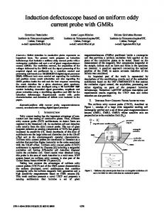
A design response spectrum is defined with two basic components: response spectral accelerations and site factors. Figure 3.1 illustrates the curve of a design spectrum using uniform seismic hazard maps based on probabilistic national ground motion mapping having a 5% chance of exceedance in 50-year for a damping ratio of 5%. For T ≤ To, the design response spectral acceleration coefficient Sa is

S a  S DS  As 

T  As To

[3.4-1]

where T

is the period of vibration in second

To  0.2TS

[3.4-2]

in which

TS 

S D1 S DS

[3.4-3]

SDS

is the short period’s (T = 0.2 second) design spectral acceleration coefficient and

SD1

is the design spectral acceleration coefficient at 1.0 second period.

These two coefficients are determined from the following equations: S DS  Fa Ss

[3.4-4]

45

Response spectral acceleration Sa

SDS

Sa 

S D1 T

SD1 As

0 To 0.2

Ts

1.0 Period T (s)

Fig. 3.1 Design response spectrum constructed using AASHTO 2009

46

S D1  Fv S1

[3.4-5]

in which Fa

is the site coefficient for 0.2 second period spectral acceleration as specified in Article 3.4.2.3 of AASHTO 2009 (Table 3.6)

Ss

is the 0.2 second period spectral acceleration coefficient on Class B rock

Fv

is the site coefficient for 1.0 second period spectral acceleration as specified in Article 3.4.2.3 of AASHTO 2009 (Table 3.7)

S1

is the 1.0 second period spectral acceleration coefficient on Class B rock.

As

is the design earthquake response spectral acceleration coefficient at the effective peak ground acceleration and is determined with

As  F pga PGA

[3.4-6]

in which Fpga

is the site coefficient for peak ground acceleration defined in Article 3.4.2.3 in AASHTO 2009, and

PGA is the peak horizontal ground acceleration coefficient on Class B rock

The design response spectral acceleration coefficient Sa is defined for the periods ranging from To to TS as follows: S a  S DS

[3.4-7]

The design response spectral acceleration coefficient Sa is defined for periods greater than TS as follows: Sa 

S D1 T

[3.4-8]

47

Values of PGA, Ss and S1 are ready to obtain from electronic versions of the ground motion maps as tabulated form of data produced by the USGS.

For T > 3 seconds, Eq. 3.4-8 seems to be conservative because of the ground motions’ closing to the constant spectral displacement range, and the design response spectral acceleration coefficient Sa is defined as

Sa 

S D1 T2

[3.4-9]

Tables 3.6 and 3.7 shows the values of site coefficients for the peak ground acceleration Fpga, short-period range Fa and for the long-period range Fv, respectively to determine the elastic seismic response coefficients of ground motion. Straight line interpolation is used to determine intermediate values of PGA, Ss and S1. For site class F site-specific geotechnical investigation and dynamic site response analyses need to be executed according to Article 3.4.3 of AASHTO 2009 specifications.

48

Table 3.6 Values of Fpga and Fa as a function of site class coefficients [Table 3.4.2.3-1, AASHTO 2009] Values of Fpga and Fa Site Class

PGA 0.10

PGA = 0.20

PGA = 0.30

PGA = 0.40

PGA  0.50

Ss  0.25

Ss = 0.50

Ss = 0.75

Ss = 1.00

Ss  1.25

A

0.8

0.8

0.8

0.8

0.8

B

1.0

1.0

1.0

1.0

1.0

C

1.2

1.2

1.1

1.0

1.0

D

1.6

1.4

1.2

1.1

1.0

E

2.5

1.7

1.2

0.9

0.9

F

-

-

-

-

-

Table 3.7 Values of Fv as a function of site class coefficient [Table 3.4.2.3-2, AASHTO 2009] Values of Fv Site Class S1  0.1

S1 = 0.2

S1 = 0.3

S1 = 0.4

S1  0.5

A

0.8

0.8

0.8

0.8

0.8

B

1.0

1.0

1.0

1.0

1.0

C

1.7

1.6

1.5

1.4

1.3

D

2.4

2.0

1.8

1.6

1.5

E

3.5

3.2

2.8

2.4

2.4

F

-

-

-

-

-

Note: Site class definition is associated with known soil properties determined by detailed site investigation. Site class definitions are specified in Table 3.8.

49

Table 3.8 Determination of site classes Site

Soil Type and Profile

Class A

Hard rock with measured shear wave velocity,  s > 5,000 ft/s

B

Rock with 2,500 ft/s <  s < 5,000 ft/s Very dense soil and soil rock with 1,200 ft/s <  s < 2,500 ft/s, or with either

C N > 50 blows/ft, or S u > 2.0 ksf

Stiff soil with 600 ft/s <  s < 1,200 ft/s, or with either 15 < N < 50 blows/ft, D or 1.0 < S u < 2.0 ksf Soil profile with  s < 600 ft/s or with either N < 15 blows/ft or S u < 1.0 ksf, E

or any profile with more than 10 ft of soft clay defined as soil with PI > 20, w > 40% and S u < 0.5 ksf. Soils requiring site-specific evaluations, such as: Peats or highly organic clays (H > 10 ft of peat or highly organic clay where H

F

is the thickness of soil) Very high plasticity clays (H > 25 ft with PI > 75) Very thick soft/medium stiff clays (H >120 ft)

50

where (in Table 3.8) s

is the average shear wave velocity for the upper 100 ft of the soil profile. The site class definitions are specified based on the upper 100 ft. of the site profile. The site profiles containing distinctly different soil layers ranges from 1 to n in the upper 100 ft. Then, the average  s for the site profile is determined by n

s 

d i 1 n

i

[3.4-10]

di  i 1  si

where n

d i 1

i

is the thickness of upper soil layers considered as 100 ft

di

is the thickness of ith soil layer in feet

n

is the total number of distinctive soil layers in the upper 100 ft of the site profile below the bridge foundation

si i N

is the shear wave velocity of ith soil layer in ft/s is any number of the distinctive soil layers between 1 and n

is the average Standard Penetration Test (SPT) blow count in blows/ft for the upper 100 ft of the soil profile and can be calculated with the following equation: n

N 

d i 1 n

i

[3.4-11]

di  i 1 N i

in which

51

Ni is the standard penetration resistance as measured directly in the field, uncorrected blow count, of ith soil layer not to exceed 100 in blows/ft

Su

is the average undrained shear strength in ksf for the upper 100 ft of the soil profile, which is determined by k

Su 

d i 1 k

i

[3.4-12]

di  i 1 Sui

where k

is the total number of cohesive soil layers in the upper 100 ft of the site profile below the bridge foundation;

Sui is the undrained shear strength of ith soil layer not to exceed 5 in ksf;

PI

is the plasticity index, and

w

is the moisture content.

52

CHAPTER 4

ANALYSIS AND COMPARISON OF ELASTIC SEISMIC RESPONSE COEFFICIENTS

4.1 COMMON PLATFORM FOR ELASTIC RESPONSE COEFFICIENT CALCULATIONS IN CODES

The elastic seismic force at the base of a structure (i.e., the elastic base shear Ve) is calculated from the basic relationship: force = mass  acceleration = weight  acceleration coefficient. In the code formats, acceleration coefficient is further modified with two multiplication factors, such as, importance factor and soil factor. As the name implies, the importance factor is an administrative factor which translates the importance of keeping the structure fully/partially operational during/after the design event into an enhanced design force from the baseline force on the basis of socio-economic demand of the structure. Soil factor is a technical factor which recognizes the fact that acceleration coefficient needs to be modified (amplified) if the soil category differs from the reference soil category. This factor used to be period independent in old codes but recent codes had adopted period dependence as a vital factor not to be ignored any more.

53

For this research, since the comparison of different spectra is made based on elastic seismic response coefficient, roles of response modification factors (R, Ro, and Rd) in NBCC [2005], CHBDC [2006] and AASHTO [2009] are irrelevant for this study and are kept beyond purview. It is noteworthy to mention that no matter which format (NBCC, AASHTO or any new format) is adopted for UHS spectrum to be used in next CHBDC edition, the usual approach of scaling elastic Csm for inelastic design remains valid. This is because spectral ordinates are meant for idealized SDOF systems (not limited to any specific real life structural system). However, for clarity of discussion, formulations of inelastic base shear calculation procedure are also included in the following sections.

The base shear calculation formulae in the seismic provisions of the three codes under this study‟s investigation are based essentially on the aforementioned principle. In this chapter, these code provisions as presented in the previous chapter will be briefly revisited, and they will be put in similar format to have a uniform basis of comparison.

4.1.1 CHBDC 2006

The elastic seismic design force at base of a structure defined as the elastic base shear Ve produced in a SDOF structural system of period T can be obtained for a site by using the following equation: Ve = Csm  W

[4.1-1]

54

The elastic acceleration coefficient used in the CHBDC [2006] is named as elastic seismic response coefficient Csm. The detailed procedure of calculating Csm is provided in the previous chapter. It should be noted that Csm can be in general described with the following equation with an upper bound limit. Csm = A  N  I  S ∕ Tk

[4.1-2]

where A

is the zonal acceleration ratio

N

is a numerical parameter to account for ground motion parameter amplification (1.2, 2.5 or 3.0)

I

is a numerical parameter to account for importance of the structure on acceleration coefficient (1.0, 1.5 or 3.0)

S

is a numerical parameter to account for soil influence on acceleration coefficient (1.0, 1.2, 1.5 or 2.0)

T

is natural period of the SDOF system

k

is the exponent of period to account for decay of Csm with increasing period (2/3 or 4/3)

The inelastic seismic design force V for the ductile structure is determined by dividing elastic design force Ve by the appropriate response modification factor R. V = Ve ∕ R = Csm  W ∕ R

[4.1-3]

55

4.1.2 NBCC 2005

The elastic base shear according to NBCC [2005] is calculated using the following equation: Ve = (Fa or Fv)  Sa(T)  Mv  I  W

[4.1-4]

where Fa

is an acceleration-related soil amplification factor

Fv

is a velocity-related soil amplification factor

Sa(T) is an uniform hazard spectral response acceleration coefficient for reference site Mv

is the higher mode factor

As evident from Eq. 4.1-4, the elastic seismic coefficient according to NBCC [2005] can be expressed as shown in Eq. 4.1-5. Csm = (Fa  Sa(T) or Fv  Sa(T))  Mv  I

[4.1-5]

Similar to CHBDC, the inelastic seismic design force V for the ductile structure is determined by dividing elastic design force Ve by the two response modification factors Ro and Rd. V = Ve ∕ (Ro  Rd) = Csm  W ∕ (Ro  Rd)

[4.1-6]

where Ro

is overstrength related force modification factor that accounts for the dependable portion of reserve strength in a structure

56

Rd

is ductility related force modification factor that reflects the capability of a structure to dissipate energy through inelastic behaviour

4.1.3 AASHTO 2009

As shown in the previous chapter, the design spectrum according to AASHTO [2009] has three components: (i) initial steep line, (ii) intermediate horizontal plateau, and (iii) nonlinear curve. The initial linear line is a function of Peak Ground Acceleration (PGA) and spectral acceleration at 0.2-second period. Horizontal line is function of spectral acceleration at 0.2-second period. Nonlinear line is the function of spectral acceleration at 1.0 second period and period T.

Therefore, the base shear calculation formulae for initial linear segment can be written in the following form: Ve = f (PGA, Fpga, Sa(0.2))  W

[4.1-7a]

or Ve = (Fa or Fv)  Sa(T)  I ∕ T k  W

[4.1-7b]

where Fpga

is the peak ground acceleration coefficient (0.8 to 2.5)

Fa(T)

is an acceleration-related soil amplification factor (0.8 to 3.5)

Fv(T)

is the velocity-related soil amplification factor (0.8 to 2.5)

Sa(T)

is the uniform hazard spectral response acceleration for reference site (at periods

57

0.2 and 1.0 second) I

is a numerical parameter to account for importance of the structure on acceleration coefficient (1.0, 1.3 or 1.5)

k

is 0 or 1

Inelastic design force V is then scaled by dividing/multiplying with appropriate factors associated with force modification and importance factor, respectively.

Elastic seismic response coefficient Csm can be deduced from Eqs. 4.1-7a and b as follows:

Csm = f (PGA, Fpga, Sa(0.2))

[4.1-8a]

or Csm = (Fa or Fv)  Sa(T)  I ∕ T k

[4.1-8b]

4.2 DESCRIPTION OF SPECTRA UNDER CONSIDERATION

The elastic design spectra for the present comparative study are constructed using common approaches of elastic seismic response coefficient Csm calculation on the basis of three code formats and using the GSC map values and/or ground motion parameters (spectral coefficients Sa(T), A and PGA) as discussed in the previous section. In the process of construction design spectra, site coefficients (Fa(T), Fv(T), S and Fpga) and importance factor I are used as per code specifications. Following notations are repeated here for the sake of clarity with reference to code specific interpretations.

58

Csm

is elastic seismic response coefficient as defined by CHBDC [2006] and AASHTO [2009].

A

is zonal acceleration ratio as defined by CHBDC [2006].

PGA

is peak ground acceleration coefficient as defined by AASHTO [2009].

Fa

is acceleration-based site coefficient as defined by NBCC [2005] and AASHTO [2009].

Fv

is velocity-based site coefficient as defined by NBCC [2005] and AASHTO [2009].

S

is site coefficient as defined by CHBDC [2006] and AASHTO [2009].

Fpga

is site coefficient for peak ground acceleration as defined by AASHTO [2009].

To have a uniform basis for comparison of design spectra, it is assumed that average shear wave velocity vavg of the soil under consideration is 760 m/s so that Fa = Fv = S = Fpga = 1.0 and I = 1.0. Following five spectral shapes are compared: a) 2%/50-yr – a spectrum that is drawn using spectral coefficients Sa(0.2), Sa(0.5), Sa(1.0) and Sa(2.0) of 4th generation seismic hazard maps with 2% probability of exceedance in 50-year according to Section 4.1.8.4 of NBCC [2005]. b) 5%/50-yr – a spectrum that is drawn using spectral coefficients Sa(0.2), Sa(0.5), Sa(1.0) and Sa(2.0) of 4th generation seismic hazard maps with 5% probability of exceedance in 50-year according to Section 4.1.8.4 of NBCC [2005].

59

c) 10%/50-yr – a spectrum that is drawn using spectral coefficients Sa(0.2), Sa(0.5), Sa(1.0) and Sa(2.0) of 4th generation seismic hazard maps with 10% probability of exceedance in 50-year according to Section 4.1.8.4 of NBCC [2005]. d) CHBDC – a spectrum that is drawn using zonal acceleration ratio A of CHBDC [2006] with 10% probability of exceedance in 50-year according to Section 4.4.7 of CHBDC [2006]. e) AASHTO – a spectrum that is drawn using spectral coefficients Sa(0.2) and Sa(1.0) of 4th generation seismic hazard maps with 5% probability of exceedance in 50-year according to Section 3.4.1 of AASHTO [2009].

4.3 INPUT SEISMIC DATA FOR ANALYSES

A total of 389 Canadian cities have been chosen for this study. These cities have been selected from the list of cities of Table A3.1.1 in CHBDC [2006]. This table contains names of cities and corresponding seismic data including zonal acceleration ratios A. Cities with zero or missing A values are excluded from this study. The reason of * this exclusion is that the denominator in the normalized C sm (defined later) become zero

* (hence infinite C sm ) which lead to „ineffective‟ statistical data. In recent time, a

comprehensive list of seismic data of spectral coefficients Sa(T) for more than 650 Canadian cities corresponding to 4th generation hazard maps at 2%/50-yr probability level has been published by Adams et al. [2003]. The longitude and latitude of the cities are also given in this publication. These information have been utilized to retrieve seismic

60

data of spectral coefficients Sa(T) and PGA at other probability levels of 5%/50-yr and 10%/50-yr for all 389 cities required for this research. This is accomplished using an online seismic hazard calculator [GSC 2009] developed by Natural Resources Canada. A sample calculation of seismic hazard calculator for Montreal is shown in Fig. 4.1. A complete listing of seismic hazard data of the selected 389 cities are saved in the text input file (spectra.in) for the computer program written for this study. The look of the input file (spectra.in) is shown in Fig. 4.2 for two cities (Abbotsford and Agassiz).

4.4 COMPUTER PROGRAM FOR ANALYSES

To manage a huge data of 389 cities and carry out associated voluminous numerical analyses, a computer program has been written for this research. The program is written in Digital Visual FORTRAN [1998] programming language. It consists of a main program (uhs.f) and several subroutines (gsc.f, aashto.f and initial.f). The program does the following tasks: – Reads all input data for 389 cities from spectra.in file and store them in array format. – Creates output files echoing input data to make sure that input data are correctly read by the program. – Calculates data for spectra construction (Csm vs. Period). * – Calculates normalized elastic seismic coefficient C sm (defined in following

section) corresponding to a set of periods.

61

Fig. 4.1 Typical calculation for one of 389 cities of online seismic hazard calculator of the GSC [2009]

62

Fig. 4.2 Partial input file of “spectra.in” containing typically formatted seismic data for Abbotsford and Agassiz of 389 cities

63

* – Does the statistical analyses from the distribution of C sm of 389 cities to examine

the trend of magnification/reduction of Csm values corresponding to those of current CHBDC [2006] along the range of period. – Writes several output files to save the aforementioned numerical results for subsequent analyses and plotting.

The results derived from running the aforementioned program are presented in the following sections in two stages: – Present and discuss the trend of the results using case examples for sixteen selected cities – Present and discuss the aggregate results based on statistical analyses using all data corresponding to 389 cities.

4.5 GENERAL FEATURES OF RESULTS BASED ON DATA FOR SIXTEEN SELECTED CITIES To have a good understanding of the relative values of elastic seismic coefficients Csm, sixteen cities (Montreal, Toronto, Saint John, Halifax, Moncton, Fredericton, TroisRivieres, Ottawa, Vancouver, Victoria, Alberni, Tofino, Prince Rupert, Kelowna, Kamloops and Inuvik), which represent seismically low to high active areas and also represent eastern and western Canada have been selected for this section. Relevant seismic data needed to represent five spectra under consideration of the sixteen cities are provided in Table 4.1. The values of zonal acceleration ratios A are taken from CHBDC

64

[2006]. The spectral coefficients Sa(T) required to illustrate UHS shapes for these cities are obtained from the aforementioned on-line seismic hazard calculator [GSC 2009] and are also shown in Table 4.1. It should be noted that for AASHTO designated Ss and S1 values are obtained from Sa(0.2) and Sa(1.0) values, respectively corresponding to 5%/50yr of Table 4.1.

The elastic seismic coefficients Csm calculated as a function of T using code specified procedures for sixteen cities are shown in Fig. 4.3 a – p. In these figures, dark blue thick solid, green dotted, light blue thin solid, black dashed and red dash-dotted lines represent spectra of 2%/50-yr, 5%/50-yr, 10%/50-yr, CHBDC and AASHTO, respectively. Following features are noted: 

A comparison among the first three spectra (2%/50-yr, 5%/50-yr and 10%/50-yr) clearly shows that lowering probability increases values of Csm about 1.53 times for spectra 2%/50-yr from that of 10%/50-yr spectra. It should be noted that these hazard maps for three probabilities use the same confidence level (50th percentile).



Sensitivity of the four spectra (2%/50-yr, 5%/50-yr, 10%/50-yr and AASHTO) is high for short periods as the rate of decay is very high for 0.2 s ≤ T ≤ 0.5 s and moderate for 0.5 s ≤ T ≤ 1.0 s in comparison to current CHBDC [2006]. For example slopes of UHS spectra are 2.1 for 0.2 s ≤ T ≤ 0.5 s whereas corresponding values are about 1.1 for standardized spectrum of CHBDC [2006]. This implies that the results of dynamic analysis are more sensitive with reference to period determination for the UHS than current CHBDC in short period range.

65

Table 4.1 Seismic data for sixteen selected cities Location Probability

Montreal, Quebec

Toronto, Ontario

2%/50-yr

5%/50-yr

10%/50-yr

2%/50-yr

5%/50-yr

10%/50-yr





0.200





0.050

PGA

0.429

0.287

0.200

0.170

0.108

0.072

Sa(0.2)

0.687

0.426

0.288

0.262

0.168

0.105

Sa(0.5)

0.340

0.201

0.127

0.126

0.077

0.050

Sa(1.0)

0.139

0.081

0.051

0.055

0.034

0.022

Sa(2.0)

0.048

0.026

0.016

0.016

0.010

0.006

A

Location

Saint John, New Brunswik

Halifax, Nova Scotia





0.100





0.050

PGA

0.225

0.132

0.090

0.122

0.080

0.057

Sa(0.2)

0.344

0.229

0.159

0.230

0.155

0.108

Sa(0.5)

0.181

0.117

0.079

0.130

0.088

0.062

Sa(1.0)

0.081

0.051

0.034

0.069

0.045

0.030

Sa(2.0)

0.025

0.016

0.011

0.020

0.013

0.009

A

Location

Moncton, New Brunswick

Fredericton, New Brunswick





0.100





0.100

PGA

0.214

0.121

0.071

0.267

0.152

0.094

Sa(0.2)

0.295

0.186

0.126

0.386

0.245

0.165

Sa(0.5)

0.160

0.102

0.070

0.205

0.128

0.086

Sa(1.0)

0.069

0.045

0.031

0.086

0.056

0.037

Sa(2.0)

0.022

0.014

0.010

0.027

0.018

0.012

A

Location

Trois-Rivieres, Quebec

Ottawa, Ontario





0.150





0.200

PGA

0.405

0.266

0.181

0.411

0.274

0.189

Sa(0.2)

0.642

0.387

0.256

0.657

0.405

0.268

Sa(0.5)

0.311

0.177

0.115

0.317

0.189

0.119

Sa(1.0)

0.125

0.073

0.045

0.132

0.079

0.049

Sa(2.0)

0.043

0.024

0.015

0.044

0.025

0.016

A

66

Table 4.1 Seismic data for sixteen selected cities (continued) Location Probability

Vancouver, British Columbia

Victoria, British Columbia

2%/50-yr

5%/50-yr

10%/50-yr

2%/50-yr

5%/50-yr

10%/50-yr





0.200





0.400

PGA

0.460

0.331

0.245

0.608

0.447

0.336

Sa(0.2)

0.927

0.665

0.489

1.217

0.892

0.671

Sa(0.5)

0.641

0.454

0.333

0.817

0.595

0.444

Sa(1.0)

0.334

0.236

0.173

0.380

0.275

0.205

Sa(2.0)

0.173

0.120

0.087

0.185

0.130

0.094

A

Location

Alberni, British Columbia

Tofino, British Columbia





0.300





0.300

PGA

0.355

0.257

0.192

0.523

0.332

0.273

Sa(0.2)

0.757

0.536

0.395

1.203

0.763

0.628

Sa(0.5)

0.559

0.380

0.292

0.937

0.595

0.489

Sa(1.0)

0.302

0.208

0.152

0.474

0.301

0.247

Sa(2.0)

0.161

0.110

0.079

0.206

0.122

0.097

A

Location

Prince Rupert, British Columbia

Kelowna, British Columbia





0.150





0.050

PGA

0.179

0.126

0.094

0.137

0.097

0.072

Sa(0.2)

0.377

0.257

0.184

0.276

0.189

0.135

Sa(0.5)

0.247

0.169

0.123

0.172

0.119

0.086

Sa(1.0)

0.150

0.106

0.078

0.094

0.068

0.051

Sa(2.0)

0.086

0.061

0.045

0.056

0.041

0.030

A

Location

Kamloops, British Columbia

Inuvik, Northwest Territories





0.050





0.050

PGA

0.138

0.097

0.071

0.062

0.045

0.035

Sa(0.2)

0.277

0.188

0.134

0.116

0.076

0.059

Sa(0.5)

0.171

0.119

0.089

0.070

0.054

0.043

Sa(1.0)

0.105

0.075

0.056

0.041

0.031

0.025

Sa(2.0)

0.062

0.044

0.033

0.026

0.020

0.016

A

67


(b) Toronto, Ontario Fig. 4.3 Comparison of elastic seismic coefficient Csm obtained from five spectra

68


(d) Halifax, Nova Scotia Fig. 4.3 Comparison of elastic seismic coefficient Csm (Continued)

69


(f) Fredericton, New Brunswick Fig. 4.3 Comparison of elastic seismic coefficient Csm (Continued)

70


(h) Ottawa, Ontario Fig. 4.3 Comparison of elastic seismic coefficient Csm (Continued)

71


(j) Victoria, British Columbia Fig. 4.3 Comparison of elastic seismic coefficient Csm (Continued)

72


(l) Tofino, British Columbia Fig. 4.3 Comparison of elastic seismic coefficient Csm (Continued)

73


(n) Kelowna, British Columbia Fig. 4.3 Comparison of elastic seismic coefficient Csm (Continued)

74


(p) Inuvik, Northwest Territories Fig. 4.3 Comparison of elastic seismic coefficient Csm (Continued)

75



The 5%/50-yr spectrum is the closest one with that of AASHTO. However, the former gives more conservative Csm values for T < 1.0 second. They share the same plateau for the peak region and the differences of Csm values along the rest of the period axis are insignificant. The similarity is simply because both spectra are constructed on the basis of the same hazard map (4th generation map with 5%/50-yr probability) and the differences (small though) are due to the application of different code formats [CHBDC 2006 and AASHTO 2009].

The scatter of other four spectra from CHBDC is noticeable. This feature will be examined in further detail in next section.

Implementation of UHS format with lowered probability in the next version of CHBDC will bring change in seismic design forces. That means it will cause increase or decrease of Csm values. To track the extent of change with reference to current CHBDC * [2006], a normalized elastic seismic coefficient ( C sm ) is obtained for each spectrum,

where: * C sm (T) = Csm-sq(T) / Csm-CHBDC(T)

[4.5-1]

where Csm-sq(T)

is the elastic seismic coefficient for a period T obtained from the spectrum in question, and

Csm-CHBDC(T)

is the elastic seismic coefficient for a period T obtained from the spectrum defined by CHBDC [2006].

76

* The C sm vs. T plots are shown in Figs. 4.4a – p. In these figures, dark blue thick

solid, green dotted, light blue thin solid, black dashed and red dash-dotted lines represent spectra of 2%/50-yr, 5%/50-yr, 10%/50-yr, CHBDC and AASHTO, respectively. As the comparison is made with reference to current CHBDC values, the horizontal black * dashed line C sm = 1.0 represents normalized spectrum of CHBDC. This is the line of

basis from which the extent of magnification or reduction is visualized for Csm(T) values * corresponding to other four spectra. For clarity of discussions, same results ( C sm vs. T)

are presented in numbers in Table 4.2. Following observations are made from these graphical and tabulated presentations: 

Current CHBDC is overly conservative as most parts of the four other spectral * lines lie way below CHBDC line ( C sm = 1.0). Table 4.2 shows that with some * exceptions at very short periods, C sm  1.0. Csm for 10%/50-yr at Montreal even

* dips down to as low as only 8% of current CHBDC value ( C sm = 0.084 at T = 4.0

seconds). The conservatism in current CHBDC is probably because of two reasons: (i) the rate of decay of Csm at intermediate to long period is proportional to 1/T 2/3  1/T 4/3 which is quite slower than theoretical estimation (1/T  1/T 2) and (ii) higher mode effects have been conservatively included in CHBDC spectrum for long periods. 

Even though hazard maps for both CHBDC [2006] and UHS spectrum 10%/50-yr * use the same probability level, C sm vs. T plots for 10%/50-yr UHS ordinates of all

* cities mostly lie below the CHBDC line C sm = 1.0. The differences are attributed

77


(b) Toronto, Ontario * Fig. 4.4 Comparison among normalized elastic seismic coefficients C sm

78


(d) Halifax, Nova Scotia * Fig. 4.4 Comparison among normalized elastic seismic coefficients C sm (Continued)

79


(f) Fredericton, New Brunswick * Fig. 4.4 Comparison among normalized elastic seismic coefficients C sm (Continued)

80


(h) Ottawa, Ontario * Fig. 4.4 Comparison among normalized elastic seismic coefficients C sm (Continued)

81


(j) Victoria, British Columbia * Fig. 4.4 Comparison among normalized elastic seismic coefficients C sm (Continued)

82


(l) Tofino, British Columbia * Fig. 4.4 Comparison among normalized elastic seismic coefficients C sm (Continued)

83


(n) Kelowna, British Columbia * Fig. 4.4 Comparison among normalized elastic seismic coefficients C sm (Continued)

84


(p) Inuvik, Northwest Territories * Fig. 4.4 Comparison among normalized elastic seismic coefficients C sm (Continued)

85

* Table 4.2 Values of normalized elastic response coefficients C sm

Montreal, Quebec

Toronto, Ontario

T 2%/50-yr 5%/50-yr 10%/50-yr AASHTO 2%/50-yr 5%/50-yr 10%/50-yr AASHTO 0.0 1.3740

0.8520

0.5760

0.5740

2.0960

1.3440

0.8400

0.8640

0.2 1.3740

0.8520

0.5760

0.8520

2.0960

1.3440

0.8400

1.3440

0.4 1.0307

0.6243

0.4087

0.4581

1.5502

0.9712

0.6183

0.7691

0.6 0.8886

0.5246

0.3314

0.4002

1.3255

0.8110

0.5264

0.6719

0.8 0.7878

0.4632

0.2923

0.3636

1.1979

0.7354

0.4768

0.6104

1.0 0.5792

0.3375

0.2125

0.3375

0.9167

0.5667

0.3667

0.5667

1.5 0.5105

0.2921

0.1829

0.2948

0.7753

0.4805

0.3058

0.4950

2.0 0.3175

0.1720

0.1058

0.2679

0.4233

0.2646

0.1587

0.4498

3.0 0.3120

0.1690

0.1040

0.2340

0.4160

0.2600

0.1560

0.3929

3.5 0.2882

0.1561

0.0961

0.2223

0.3842

0.2401

0.1441

0.3732

4.0 0.2520

0.1365

0.0840

0.2126

0.3360

0.2100

0.1260

0.3570

Saint John, New Brunswick

Halifax, Nova Scotia

0.0 1.3760

0.9160

0.6360

0.2500

1.8400

1.2400

0.8640

0.1250

0.2 1.3760

0.9160

0.6360

0.2500

1.8400

1.2400

0.8640

0.1250

0.4 1.0647

0.6982

0.4780

0.2210

1.4778

0.9983

0.6997

0.1105

0.6 0.9544

0.6153

0.4150

0.1687

1.3967

0.9414

0.6592

0.0843

0.8 0.8690

0.5558

0.3734

0.1392

1.3415

0.8934

0.6147

0.0696

1.0 0.6750

0.4250

0.2833

0.1200

1.1500

0.7500

0.5000

0.0600

1.5 0.5787

0.3658

0.2457

0.0916

0.9719

0.6333

0.4259

0.0458

2.0 0.3307

0.2117

0.1455

0.0756

0.5291

0.3439

0.2381

0.0378

3.0 0.3250

0.2080

0.1430

0.0577

0.5200

0.3380

0.2340

0.0288

3.5 0.3002

0.1921

0.1321

0.0521

0.4803

0.3122

0.2161

0.0260

4.0 0.2625

0.1680

0.1155

0.0476

0.4200

0.2730

0.1890

0.0238

86

* Table 4.2 Values of normalized elastic response coefficients C sm (Continued)

Moncton, New Brunswick

Fredericton, New Brunswick


0.7440

0.5040

0.2500

1.5440

0.9800

0.6600

0.2500

0.2 1.1800

0.7440

0.5040

0.2500

1.5440

0.9800

0.6600

0.2500

0.4 0.9274

0.5881

0.4011

0.2210

1.2004

0.7555

0.5082

0.2210

0.6 0.8406

0.5371

0.3687

0.1687

1.0742

0.6734

0.4517

0.1687

0.8 0.7569

0.4869

0.3347

0.1392

0.9594

0.6090

0.4065

0.1392

1.0 0.5750

0.3750

0.2583

0.1200

0.7167

0.4667

0.3083

0.1200

1.5 0.4968

0.3221

0.2239

0.0916

0.6170

0.4040

0.2675

0.0916

2.0 0.2910

0.1852

0.1323

0.0756

0.3572

0.2381

0.1587

0.0756

3.0 0.2860

0.1820

0.1300

0.0577

0.3510

0.2340

0.1560

0.0577

3.5 0.2641

0.1681

0.1201

0.0521

0.3242

0.2161

0.1441

0.0521

4.0 0.2310

0.1470

0.1050

0.0476

0.2835

0.1890

0.1260

0.0476

Trois Revieres, Quebec

Ottawa, Ontario

0.0 1.7120

1.0320

0.6827

0.3750

1.3140

0.8100

0.5360

0.5000

0.2 1.7120

1.0320

0.6827

0.3750

1.3140

0.8100

0.5360

0.5000

0.4 1.2707

0.7450

0.4886

0.3316

0.9734

0.5904

0.3815

0.4421

0.6 1.0821

0.6173

0.3992

0.2530

0.8299

0.4950

0.3112

0.3374

0.8 0.9547

0.5487

0.3495

0.2089

0.7397

0.4417

0.2765

0.2785

1.0 0.6944

0.4056

0.2500

0.1800

0.5500

0.3292

0.2042

0.2400

1.5 0.6115

0.3531

0.2184

0.1374

0.4805

0.2839

0.1774

0.1832

2.0 0.3792

0.2117

0.1323

0.1134

0.2910

0.1654

0.1058

0.1512

3.0 0.3727

0.2080

0.1300

0.0865

0.2860

0.1625

0.1040

0.1154

3.5 0.3442

0.1921

0.1201

0.0781

0.2641

0.1501

0.0961

0.1041

4.0 0.3010

0.1680

0.1050

0.0714

0.2310

0.1312

0.0840

0.0952

87


Vancouver, British Columbia

Victoria, British Columbia


1.3300

0.9780

0.6620

1.2170

0.8920

0.6710

0.4470

0.2 1.8540

1.3300

0.9780

1.3300

1.2170

0.8920

0.6710

0.8920

0.4 1.6656

1.1860

0.8709

1.3346

1.0748

0.7849

0.5877

0.7776

0.6 1.7180

1.2165

0.8922

1.1659

1.0813

0.7870

0.5872

0.6793

0.8 1.6402

1.1605

0.8510

1.0593

0.9961

0.7235

0.5397

0.6172

1.0 1.3917

0.9833

0.7208

0.9833

0.7917

0.5729

0.4271

0.5729

1.5 1.3841

0.9719

0.7098

0.8590

0.7712

0.5528

0.4081

0.5005

2.0 1.1443

0.7937

0.5754

0.7805

0.6118

0.4299

0.3109

0.4547

3.0 1.1245

0.7800

0.5655

0.6818

0.6013

0.4225

0.3055

0.3972

3.5 1.0385

0.7204

0.5223

0.6477

0.5553

0.3902

0.2821

0.3773

4.0 0.9082

0.6300

0.4567

0.6195

0.4856

0.3412

0.2467

0.3609

Alberni, British Columbia

Tofino, British Columbia

0.0 1.0093

0.7147

0.5267

0.7500

1.6040

1.0173

0.8373

0.7500

0.2 1.0093

0.7147

0.5267

0.7500

1.6040

1.0173

0.8373

0.7500

0.4 0.9425

0.6515

0.4921

0.6631

1.5467

0.9817

0.8073

0.6631

0.6 1.0030

0.6829

0.5217

0.5061

1.6686

1.0596

0.8706

0.5061

0.8 0.9690

0.6626

0.4979

0.4177

1.5780

1.0021

0.8230

0.4177

1.0 0.8389

0.5778

0.4222

0.3600

1.3167

0.8361

0.6861

0.3600

1.5 0.8426

0.5787

0.4204

0.2747

1.2376

0.7698

0.6261

0.2747

2.0 0.7099

0.4850

0.3483

0.2268

0.9083

0.5380

0.4277

0.2268

3.0 0.6977

0.4767

0.3423

0.1731

0.8927

0.5287

0.4204

0.1731

3.5 0.6443

0.4402

0.3162

0.1562

0.8244

0.4883

0.3882

0.1562

4.0 0.5635

0.3850

0.2765

0.1429

0.7210

0.4270

0.3395

0.1429

88


Prince Rupert, British Columbia

Kelowna, British Columbia


0.6853

0.4907

0.3750

2.2080

1.5120

1.0800

0.1250

0.2 1.0053

0.6853

0.4907

0.3750

2.2080

1.5120

1.0800

0.1250

0.4 0.8757

0.5982

0.4323

0.3316

1.8699

1.2878

0.9259

0.1105

0.6 0.8995

0.6181

0.4505

0.2530

1.8543

1.2900

0.9366

0.0843

0.8 0.9039

0.6281

0.4596

0.2089

1.7982

1.2697

0.9336

0.0696

1.0 0.8333

0.5889

0.4333

0.1800

1.5667

1.1333

0.8500

0.0600

1.5 0.8590

0.6079

0.4477

0.1374

1.6380

1.1903

0.8845

0.0458

2.0 0.7584

0.5380

0.3969

0.1134

1.4816

1.0847

0.7937

0.0378

3.0 0.7454

0.5287

0.3900

0.0865

1.4561

1.0660

0.7800

0.0288

3.5 0.6884

0.4883

0.3602

0.0781

1.3447

0.9845

0.7204

0.0260

4.0 0.6020

0.4270

0.3150

0.0714

1.1759

0.8609

0.6300

0.0238

Kamloops, British Columbia

Inuvik, Northwest Territories

0.0 2.2160

1.5040

1.0720

0.1250

0.9280

0.6080

0.4720

0.1250

0.2 2.2160

1.5040

1.0720

0.1250

0.9280

0.6080

0.4720

0.1250

0.4 1.8669

1.2848

0.9410

0.1105

0.7721

0.5549

0.4373

0.1105

0.6 1.8709

1.3066

0.9770

0.0843

0.7612

0.5857

0.4671

0.0843

0.8 1.8873

1.3300

0.9939

0.0696

0.7555

0.5774

0.4625

0.0696

1.0 1.7500

1.2500

0.9333

0.0600

0.6833

0.5167

0.4167

0.0600

1.5 1.8236

1.2995

0.9719

0.0458

0.7316

0.5569

0.4477

0.0458

2.0 1.6403

1.1641

0.8731

0.0378

0.6879

0.5291

0.4233

0.0378

3.0 1.6121

1.1440

0.8580

0.0288

0.6760

0.5200

0.4160

0.0288

3.5 1.4888

1.0566

0.7924

0.0260

0.6243

0.4803

0.3842

0.0260

4.0 1.3019

0.9239

0.6930

0.0238

0.5460

0.4200

0.3360

0.0238

89

to the difference of confidence levels i.e., 50th and 84th percentiles used for 4th generation hazard and CHBDC [2006] maps, respectively. This is consistent with the observations made by Heidebrecht [1997, 1999] that the ratios of 4th generation hazard values of 84th and 50th percentiles vary in the range of 1.5 to 3.0. The differences are more pronounced in long period than short periods. The * * differences also vary significantly from city to city ( C sm = 0.84 to 0.13, C sm = 0.58

* * to 0.08, C sm = 0.98 to 0.46 and C sm = 0.67 to 0.25, for Toronto, Montreal,

Vancouver and Victoria, respectively). This clearly highlights the fact that 4th generation hazard map with 10%50-yr should not be used for next CHBDC edition. 

* For very short period, C sm of 2%/50-yr varies from 1.0 to 2.2. That means if the

UHS spectrum (2%/50-yr) is to be adopted for next CHBDC edition, there will be significant increase in elastic seismic design force from current CHBDC force for very short period. And, there will be strong argument against this increment as poor performances of bridges are probably not known under past seismic events in Canada to support such change. A corrective factor can be applied to bring the design force values to the current CHBDC values for short period range. 

Fig. 4.3 and Table 4.2 suggest that 5%/50-yr is a preferred one among the four options as (i) increase of design seismic force for short period zone is not very high and (ii) it is very close to AASHTO values (i.e., NBCC 2005 and AASHTO 2009 formats are very similar). To allay the fear of too low design seismic force

90

for intermediate and long periods, a compromising calibration factor should be used.

With reference to current CHBDC provision, the nature of magnification and reduction of base shear corresponding to the four spectra varies dramatically from city to city. To have a statistically convincing conclusion a broad based study is conducted in the next section.

4.6 STATISTICAL INFERENCE FROM RESULTS BASED ON DATA FOR 389 CITIES It is evident from the discussion of previous section that no generally applicable conclusion can be drawn from the results obtained from the limited scope of evaluation of * * Csm and/or C sm based on sixteen cities. The magnification/reduction of C sm corresponding

to the same spectrum varies dramatically from city to city. To apprehend a complete picture and to have a statistically convincing inference, seismic data corresponding to 389 cities (with usable data) are brought under examination in this section.

* * To track the distribution C sm data in the C sm vs. T diagram for the four spectra

* (viz., 2%/50-yr, 5%/50-yr, 10%/50-yr and AASHTO), C sm vs. T diagrams are plotted in

Figs. 4.5 to 4.8. For visual clarity, the period range has been divided into five segments: (i) Period Range 1: T = 0 s to 0.5 s, (ii) Period Range 2: T = 0.5 s to 1.0 s, (iii) Period Range 3: T = 1.0 s to 2.0 s, (iv) Period Range 4: T = 2.0 s to 4.0 s and (v) Period Range 5: T = 4.0 s to 5.0 s.

91

* Figs. 4.5 (a), (b), (c), (d) and (e) plot the distribution of C sm data corresponding to

2%/50-yr spectrum for Period Ranges 1, 2, 3, 4 and 5, respectively. From these figures, it * is evident that in the short period range, most of the data lies above the C sm = 1.0 line.

The extents of variation of base shear for most of the cities are in the range of 90% – 200% and 40% – 140% for short and long period ranges, respectively. There is a general trend of less magnification with increasing period. The maximum magnification or reduction goes as high as 6 times and as low as 0.4 times, respectively.


5%/50-yr spectrum for Period Range 1, 2, 3, 4 and 5, respectively. From these figures, it * is evident that in the short period range, majority of the data lies below the C sm = 1.0 line.

The extents of variation of base shear for most of the cities are in the ranges of 60% – 200% and 30% – 110% for short and long period ranges, respectively. There is a general trend of less magnification with increasing period. The maximum magnification or reduction attains as high as 4 times and as low as 0.1 time, respectively.


10%/50-yr spectrum for Period Range 1, 2, 3, 4 and 5, respectively. From these figures, it * is evident that most of the data lies below the C sm = 1.0 line. The extents of variation of

base shear for most of the cities are in the range of 40% – 100% and 20% – 80% for short and long period ranges, respectively. There is a general trend of less magnification with increasing period. The maximum magnification or reduction achieves as high as 3 times and as low as 0.1 time, respectively.

92

* Fig. 4.5(a) Distribution of normalized elastic seismic coefficient C sm for 2%/50-yr

spectrum of 389 cities (Period Range 1: 0 to 0.5 seconds)

93

* Fig. 4.5(b) Distribution of normalized elastic seismic coefficient C sm for 2%/50-yr

spectrum of 389 cities (Period Range 2: 0.5 to 1.0 second)

94

* Fig. 4.5(c) Distribution of normalized elastic seismic coefficient C sm for 2%/50-yr

spectrum of 389 cities (Period Range 3: 1.0 to 2.0 seconds)

95

* Fig. 4.5(d) Distribution of normalized elastic seismic coefficient C sm for 2%/50-yr


96

* Fig. 4.5(e) Distribution of normalized elastic seismic coefficient C sm for 2%/50-yr


97



98



99



100



101



102



103



104



105



106



107


AASHTO spectrum for Period Range 1, 2, 3, 4 and 5, respectively. From these figures, it * is evident that majority of the data lies below the C sm = 1.0 line. The extents of variation

of base shear for most of the cities are in the range of 50% - 150% and 20% - 90% for short and long period ranges, respectively. There is a general trend of less magnification with increasing period. The maximum magnification or reduction attains as high as 5 times and as low as 0.1 time, respectively.

The graphical representations in Figs. 4.5 to 4.8 of the computer analyses results * lack clear visibility as very often, many data are overlapped in the C sm vs. T plots. To

have a clear view, a tabulated format of the graphical interpretation of the computer analyses results is reproduced in Fig. 4.9. It shows the percentage of data where a specific * spectrum produces C sm < n.n value. For example, in the period range 2.0 to 4.0 s, 70.6%

of total data (i.e., 5767 data out of 8169 data) will have less than 50% base shear of * current CHBDC level (as C sm < 0.5 for 5767 data) according to the 2%/50-yr spectrum. It

should be noted that for each city, the computer program generates 21 data (21 spectral * coefficients and hence 21 data of C sm from 2.0 s to 4.0 s with increment of 0.1 s) in this

period range. The total number of data for 2.0 to 4.0 s period range, therefore, becomes 21389 = 8169 data. This translates that about 275 cities out of 389 cities will have less * than 50% base shear of current CHBDC level (as C sm < 0.5) incorporating to the 2%/50-

yr spectrum. Similarly, roughly about 321 (82.4%), 342 (87.9%) and 303 (78%) cities out of 389 cities will have less than 50% base shear of current CHBDC level according to the 5%/50-yr, 10%/50-yr and AASHTO spectra, respectively.

108

* Fig. 4.8(a) Distribution of normalized elastic seismic coefficient C sm for AASHTO


109

* Fig. 4.8(b) Distribution of normalized elastic seismic coefficient C sm for AASHTO


110

* Fig. 4.8(c) Distribution of normalized elastic seismic coefficient C sm for AASHTO


111

* Fig. 4.8(d) Distribution of normalized elastic seismic coefficient C sm for AASHTO


112

* Fig. 4.8(e) Distribution of normalized elastic seismic coefficient C sm for AASHTO


113

* Another indicator to trace the trend of the C sm is provided in Fig. 4.9 with the

mean value of the data corresponding to the specific period range. The mean values of * C sm data of 5%/50-yr spectrum are 0.9, 0.71, 0.51, 0.35 and 0.35 for 0-0.5, 0.5-1.0, 1.0-

2.0, 2.0-4.0 and 4.0-5.0 seconds period ranges, respectively. A clear trend of significant reduction of base shear from the current CHBDC provisions can be identified with increasing period. Since, AASHTO uses same hazard maps with 5%/50-yr spectrum, a close proximity of the mean values (0.89, 0.66, 0.52, 0.41 and 0.39) are noted even though the two spectra use different formats.

Significant reduction of the base shear for 10%/50-yr spectrum from current CHBDC provision is predicted as the mean value varies from 0.62 to 0.24. This makes the 10%/50-yr spectrum an impractical option for the next CHBDC edition. In other words, even though current CHBDC [2006] uses the same probability level for hazard maps (10% probability of exceedance in 50 years) with that of 10%/50-yr spectrum, the magnitude of reduction of Csm clearly indicates that current CHBDC provision is very conservative. The degree of conservatism is low for the short period range because the „standardized spectrum‟ is based on zero period control point (zonal velocity ratio A of CHBDC, 2006). With increasing period, the degree of inaccuracy increases in the „standardized spectrum‟. Table 4.3 shows percentage of data (i.e., cities) that fall within 10% of current CHBDC [2006] base shear value. As evident, quite a low percentage of data (20% to 1%) lie in this bandwidth. In other words, for most of the data (80% to 99%), increase or decrease of base shear values falls outside this range. It suggests that if any one of the

114

* * Fig. 4.9 Computer output of percentage of C sm  n.n data in the C sm vs. T diagrams for

four spectra

Table 4.3 Percentage of cities 10% base shear change from current CHBDC level * Percentage (%) of data in preferred band width 0.9 ≥ C sm ≤ 1.1

Spectrum

Range 1

Range 2

Range 3

Range 4

Range 5

0 to 0.5 s

0.5 to 1.0 s

1.0 to 2.0 s

2.0 to 4.0 s

4.0 to 5.0 s

2%/50-yr

16.3

18.5

11.4

4.8

5.2

5%/50-yr

17.6

10.2

4.8

2

1.9

10%/50-yr

7.9

2.4

1.2

0.9

1.1

AASHTO

18.5

7.5

2.5

1

0.7

115

four spectra is adopted for CHBDC, with reference to the base shear, a dramatic change will be enforced to current provision. Therefore, none of the four spectra can be adopted in the present shapes for the next CHBDC edition. That issue is addressed in the next chapter.

116

CHAPTER 5

PROPOSED SPECTRAL FORMAT

5.1 INTRODUCTION

The inadequacies and shortfalls of the four spectral formats (i.e, 2%/50-yr, 5%/50-yr, 10%/50-yr and AASHTO) demand modification of the spectral formats for CHBDC application. Among them the 10%/50-yr spectrum is dropped from current investigation as its difference with current CHBDC [2006] is too large for modification. This chapter introduces new formats of the proposed spectra, viz., modified 2%/50-yr, modified 5%/50-yr, and modified AASHTO. A program described in the previous chapter is also prepared to determine the optimum values of the modification factors incorporated into the three spectral formats. Thus, the chapter presents the strategies of modifying the three spectral formats. Finally, a recommendation is made for the most suitable spectral format for next CHBDC edition.

117

5.2 GENERAL TREND OF DESIGN SPECTRA BASED ON 4TH GENERATION SEISMIC HAZARD MAPS

The statistical analyses using the seismic hazard data of 389 cities in the previous chapter well demonstrated the fact that none of the uniform hazard spectral formats based on 4th generation seismic hazard maps (2%/50-yr, 5%/50-yr, 10%/50-yr and AASHTO) * produces consistent results in terms of normalized elastic response coefficient ( C sm )

across the geographical boundary of application as well as across the range of period. The major concern of using the 4th generation seismic hazard maps is that the resultant base shear will be very low irrespective of period range based on 4th generation hazard maps compared to current level. The implication here is that the seismic hazard maps of CHBDC [2006] and NBCC [1995] are ‘very conservative’. It is also noteworthy that the degree of conservatism is not constant with period and varies with period and probability level. Any new spectral format based on 4th generation seismic hazard maps (of any probability levels under consideration) is bound to reduce the magnitude of base shear values from the current CHBDC [2006] level for most of the cases. There will be a huge discomfort to adopt the 4th generation seismic hazard maps in the CHBDC with such prospects because the historical performances of thousands of bridges which have been designed and constructed during last several decades in Canada do not have any noticeable records of poor performances during and after the seismic events occurred. Such history of satisfactory performance of bridges in Canada does not permit big change in the level of current base shear. On the other hand, the 4th generation seismic hazard maps are based on enriched inventory of seismic data/events, better hazard modeling techniques and significant progress on ground motion characterization. The same is true

118

for uniform hazard spectral format. Adoption of these two important facets of seismic engineering development into CHBDC is inevitable and unavoidable. To that end, this study proposes some modification of the 2%/50-yr, 5%/50-yr and AASHTO formats and establishes the validity of such modification.

5.3 APPROACH FOR SPECTRA MODIFICATION

Present analysis is focused on introducing and applying modification factors to * the code specified formats that will bring improvement of C sm distribution corresponding

* to 389 Canadian cities in the C sm vs. T diagram. As this study is in search of a UHS

spectrum in a modified format that does not bring a radical change in the magnitude of * current CHBDC base shear level (i.e., no large magnification/reduction of C sm ), the

* objective of this research is to find a spectrum for which most of the C sm data lie in the

* vicinity of C sm = 1.0 line.

To achieve those objectives, the general approach of modifying uniform hazard spectral format of the two codes (NBCC and AASHTO) is focused on (i) having * maximum data in the preferred bandwidth of 0.9 ≤ C sm ≤ 1.5 and (ii) having minimum

* data below the C sm = 0.9 level. The implication here is twofold:

i) Adopt conservative approach: Maximize data in the preferred bandwidth so that the base shear values corresponding to the modified spectra neither derive too much increase (more than

119

50%) nor derive too much decrease (less than 10%) of current CHBDC base shear level, and ii) Avoid unsafe data: Do not allow too much data that will result low base shear (less than 10% of * current CHBDC level) to remain in the unsafe zone ( C sm < 0.9).

The points of the approach adopted in this study for modifying the code specified * spectral format with reference to relative position of C sm distribution are illustrated in

Fig. 5.1.

5.4 MODIFICATION OF NBCC 2005 UHS FORMAT WITH 2%/50-YR HAZARD MAPS The 2%50-yr spectrum in UHS format as defined in the previous chapter uses a linear interpolation and extrapolation of four spectral ordinates viz., Sa(0.2), Sa(0.5), Sa(1.0) and Sa(2.0). These amplitudes are in need of reduction or magnification to fit the goal described above. To that end, four modification factors (FT) are introduced as follows: F0.2 = Multiplying factor for Sa(0.2) F0.5 = Multiplying factor for Sa(0.5) F1.0 = Multiplying factor for Sa(1.0) F2.0 = Multiplying factor for Sa(2.0)

The main features of 2%/50-yr spectrum remain the same as described in chapter 3.

120

* C sm

Too much increase of base shear 1.5 Acceptable increase of base shear nservative range Acceptable decrease of base shear

1.0 0.9

Too much decrease of base shear

Period T

* Fig. 5.1 Schematic representation of expected distribution of C sm for the modified UHS

spectrum

121

With the modification factors, the modified spectrum takes the shape as follows: for period, T = 0.2 s, S(T) = F0.2 FaSa(0.2)

[5.4-1]

for period, T = 0.5 s, the smallest value from the following two equations is to be taken: S(T) = F0.5FvSa(0.5)

[5.4-2]

or S(T) = F0.2 FaSa(0.2)

[5.4-3]

for period, T = 1.0 s, S(T) = F1.0 FvSa(1.0)

[5.4-4]

for period, T = 2.0 s, S(T) = F2.0 FvSa(2.0)

[5.4-5]

for period range 4.0 s or more, S(T) = F2.0 FvSa(2.0)/2

[5.4-6]

5.5 COMPUTER PROGRAM FOR ANALYSES

The program presented previously in chapter 4 is modified with an eventual goal to obtain optimum values of the modification factors and to establish the validity of the modified spectrum. Detailed presentation of the modified source codes will largely be unnecessary duplication and hence not presented here. The program accomplishes similar tasks as described in chapter 4.

122

5.6 MODIFICATION FACTORS FOR 2%/50-YR SPECTRUM

The modification factors those have been introduced above have significant impact on the base shear values. Obtaining optimum modification factors requires iterative analyses similar to the statistical analyses presented in the previous chapter. For the current purpose, the computer program was modified to accommodate the roles of four modification factors and corresponding statistical analyses were conducted. Figure 5.2 shows an output results of the first execution of the computer program (Run 1) for * distribution of C sm data without any modification as specified for 2%/50-yr spectrum

(i.e., F0.2 = F0.5 = F1.0 = F2.0 = 1.0). It is observed in this figure that the amount of ‘unsafe’ * data for C sm < 0.9 is unacceptably high (16.7%, 43.5%, 72.2%, 85.4% and 85.4% for

* Period Ranges 1, 2, 3, 4 and 5, respectively). The percentage of data for 0.9 ≤ C sm ≤ 1.5

are 51.3%, 42.2%, 13.5%, 11.2% and 11.4% corresponding to Period Ranges 1, 2, 3 and 4, respectively. That means the 2%/50-yr spectrum produces unacceptable results especially in the longer period ranges. The same fact is reflected with the low values of * mean C sm (0.79, 0.54 and 0.53) for the last three period ranges.

The above interpretation of computer program output indicates that in order to modify the 2%/50-yr spectrum and to meet the present purpose, two things should be done:

i)

Reduce the spectral amplitudes at 0.2-second period (i.e., find a value of F0.2 where F0.2 < 1.0), and

123

ii)

Increase the spectral amplitudes at periods of 0.5, 1.0 and 2.0 seconds (i.e., find values of F0.5, F1.0 and F2.0 where F0.5 > 1.0, F1.0 > 1.0 and F2.0 > 1.0).

Finding the optimum values for the modification factors have been conducted through iterative runs of the computer program and has been described in the following sections.

The second trial execution (Run 2) is performed taking the first modification factor F0.2 = 0.9 and other factors are kept equal to unity F0.5 = F1.0 = F2.0 = 1.0. The results obtained from the execution of the program are shown in Fig. 5.3. A close examination on the results of the Runs (compare results shown in Figs. 5.2 and 5.3) shows clear signs of improvement and has been highlighted in Table 5.1. Percentage of * data distributed in the preferred bandwidth (0.9 ≤ C sm ≤ 1.5) has increased from 51.3% to

* 53.7% and percentage of data below C sm = 1.5 has also increased from 68% to 74.6%.

However, since the spectrum has been lowered in the short period zone, the amount of * data below C sm = 0.9 line has also increased (16.7% to 20.9%) which in fact has gone in

the opposite direction we are looking for. But that negativity can be addressed by increasing spectral amplitudes at other three control points.

Results of a subsequent execution (Run 3) is shown in Fig. 5.4 where F0.5 is raised to 1.1 from 1.0 and other factors are kept unchanged as those of Run 2 (i.e., F1.0 = 0.9 and F1.0 = F2.0 = 1.0). As expected, the previous negativity has disappeared (data for * C sm < 0.9 has improved from 20.9% to 16.0%, i.e., more data are on the conservative

* side). Data in the preferred bandwidth (0.9 ≤ C sm ≤ 1.5) also increased from 53.7% to

124

* Fig. 5.2 Computer Program Run 1: Distribution of C sm with all modification factors

FT = 1.0 (2%/50-yr spectrum)

* Fig. 5.3 Computer Program Run 2: Distribution of C sm with

F0.2 = 0.9, F0.5 = F1.0 = F2.0 = 1.0 (2%/50-yr spectrum)

* Fig. 5.4 Computer Program Run 3: Distribution of C sm with F0.2 = 0.9, F0.5 = 1.1,

F1.0 = F2.0 = 1.0 (2%/50-yr spectrum)

125

Table 5.1 Comparison between Run 1 and Run 2 corresponding to Figures 5.2 and 5.3 Influence of F0.2 on Period Range 1 (T = 0 to 0.5 s) Values of Modifiers

F0.2 = 1.0 and F0.5 = F1.0 = F2.0 = 1.0 F0.2 = 0.9 and F0.5 = F1.0 = F2.0 = 1.0

* 0.9 ≤ C sm ≤ 1.5

* C sm < 0.9

* C sm ≤ 1.5

Mean

51.3%

16.7%

68%

1.38

53.7%

20.9%

74.6%

1.29

Table 5.2 Comparison between Run 2 and Run 3 corresponding to Figures 5.3 and 5.4 Influence of F0.2 on Period Range 1 (T = 0 to 0.5 s) Values of modifiers

F0.2 = 0.9, F0.5 = 1.0 and F1.0 = F2.0 = 1.0 F0.2 = 0.9, F0.5 = 1.1 and F1.0 = F2.0 = 1.0

* 0.9 ≤ C sm ≤ 1.5

* C sm < 0.9

* C sm ≤ 1.5

Mean

53.7%

20.9%

74.6%

1.29

56.4%

16.0%

72.4%

1.33

126

56.4%. The other two indicators, however, have shown insignificant changes (Table 5.2).

Discussion of results obtained from three executions displays the necessity of more computer program executions to obtain the optimum values of the modification factors. To that end, a set of modification trial factors have been used and corresponding * percentage of data in the preferred band width (0.9 ≤ C sm ≤ 1.5) has been recorded. The

results are then tabulated in Table 5.3 and are plotted as shown in Fig. 5.5. It is clear from Fig. 5.5 that the optimum values of modification factors are: F0.2 = 0.8, F0.5 = 1.1, F1.0 = 1.5 and F2.0 = 4.0 that produce maximum percentage of data in the preferred bandwidth.

The performance of the modification factors are also recorded with reference to * the second criterion viz., percentage of data in the C sm < 0.9 in Table 5.4 and

corresponding graphical plot is presented in Fig. 5.6. As expected, a general trend is obvious that with increasing values of modification factors, percentage of data in the * C sm < 0.9 zone reduces. However, the rate of decrement does not change significantly as

the modification factors reach the optimum values. Therefore, reading Fig. 5.6 in association of Fig. 5.5 endorses the validity of the optimum modification factors obtained from Fig. 5.5.

It should be noted that to trace the performance of modification factors, F0.2, F0.5, F1.0 and F2.0, the data in the Period Ranges 1, 2, 3 and 4 are considered to be directly influenced. This consideration has been the basis of developing Tables 5.3, 5.4 and Figs. 5.5 and 5.6.

127

Fig. 5.5 Defining optimum modifiers from iterative program executions for 2%/50-yr spectrum with reference to first criterion

Fig. 5.6 Defining optimum modifiers from iterative program executions for 2%/50-yr spectrum with reference to second criterion

128

* Table 5.3 C sm distribution pattern with decreasing values of modification factors for * 2%/50-yr spectrum with reference to preferred bandwidth (0.9 ≤ C sm ≤ 1.5)

* 0.9 ≤ C sm ≤ 1.5

F0.2

% of data

F0.5

% of data

F1.0

% of data

F2.0

% of data

1.2

35

1.2

43

0.9

58

1

11

1.1

41

1.3

44

1

61

2

19

1

47

1.4

41

1.5

66

2.5

34

0.9

53

1.5

39

2

60

3

44

0.8

57

1.1

49

2.5

51

4

45

0.7

55

1

48

3

42

4.5

37

0.9

47

5

25

0.8

45

* Table 5.4 C sm distribution pattern with decreasing values of modification factors for * 2%/50-yr spectrum with reference to C sm < 0.9

* C sm < 0.9

F0.2

% of data

F0.5

% of data

F1.0

% of data

F2.0

% of data

1.2

4.3

1.2

5.2

0.9

29.4

1

85.4

1.1

5.6

1.3

4.1

1

25

2

63.2

1

6.9

1.4

3.2

1.5

7.9

2.5

45.1

0.9

9.3

1.5

2.5

2

1.4

3

26.2

0.8

13.4

1.1

8.3

2.5

0.9

4

3.5

0.7

24.8

1

13.1

3

0.4

4.5

1.6

0.9

18.3

5

1

0.8

24.4

129

After obtaining the optimum values of the modification factors, the program is executed (Run 4) to calculate the final results, which are presented in Fig. 5.7. The comparison between the original 2%/50-yr spectrum (i.e., NBCC [2005] specified UHS using 2%/50-yr hazard map) and the modified spectrum is presented in tabulated form in Table 5.5. An obvious and significant improvement of the modified spectrum is visible in this table. The improvement is marked with distinct increase of data in the preferred * bandwidth (0.9 ≤ C sm ≤ 1.5) and significant decrease of data in the unsafe range

* ( C sm < 0.9). This establishes the validity and superiority of the modified spectrum without

reservation.

An example of excellent outcome of the modified spectrum for Montreal is shown in Figs. 5.8 (a) and (b). The detail results for all of 389 cities are presented in Figs. 5.9 (a) to (e) divided into five period ranges. It is observed that there are some cases of excessive magnification. However, their share to the total number of cases is insignificant. They should be considered as aberrant cases and do not have influence on the general findings of this study.

5.7 MODIFICATION OF NBCC 2005 UHS FORMAT WITH 5%/50-YR HAZARD MAPS Similar steps are followed to obtain the optimum modification factors for modified 5%/50-yr spectrum as defined in previous section. Figure 5.10 shows an output * results of first computer program execution (Run 1) for distribution of C sm data without

130

* Fig. 5.7 Computer Program Run 4: Distribution of C sm with F0.2 = 0.8, F0.5 = 1.1,

F1.0 = 1.5 and F2.0 = 4.0 (2%/50-yr spectrum)


Spectrum

2%/50-yr – NBCC spectrum Modified spectrum 2%/50-yr – NBCC spectrum Modified spectrum 2%/50-yr – NBCC spectrum Modified spectrum 2%/50-yr – NBCC spectrum Modified spectrum 2%/50-yr – NBCC spectrum Modified spectrum

Values of Modifiers

* Influence of Modification Factors on C sm Distribution * * C sm 0.9 ≤ C sm ≤ 1.5 < 0.9

Period Range 1: 0 to 0.5 s F0.2 = F0.5 = F1.0 = 51.3% F2.0 = 1.0 F0.2 = 0.8, F0.5 = 1.1, 57.9% F1.0 = 1.5, F2.0 = 4.0 Period Range 2: 0.5 to 1.0 s F0.2 = F0.5 = F1.0 = 42.2% F2.0 = 1.0 F0.2 = 0.8, F0.5 = 1.1, 51.4% F1.0 = 1.5, F2.0 = 4.0 Period Range 3: 1.0 to 2.0 s F0.2 = F0.5 = F1.0 = 13.5% F2.0 = 1.0 F0.2 = 0.8, F0.5 = 1.1, 61.7% F1.0 = 1.5, F2.0 = 4.0 Period Range 4: 2.0 to 4.0 s F0.2 = F0.5 = F1.0 = 11.2% F2.0 = 1.0 F0.2 = 0.8, F0.5 = 1.1, 45.1% F1.0 = 1.5, F2.0 = 4.0 Period Range 5: 4.0 to 5.0 s F0.2 = F0.5 = F1.0 = 11.1% F2.0 = 1.0 F0.2 = 0.8, F0.5 = 1.1, 45.6% F1.0 = 1.5, F2.0 = 4.0

131

16.7% 21.3%

43.5% 18.2%

72.2% 7.9%

85.4% 3.5%

85.4% 3.5%



Fig. 5.8 Comparison between modified 2%/50-yr and CHBDC 2006 spectra

132

* Fig. 5.9(a) Distribution of normalized elastic seismic coefficient C sm for modified

2%/50-yr spectrum of 389 cities (Period Range 1: 0 to 0.5 seconds)

133

* Fig. 5.9(b) Distribution of normalized elastic seismic coefficient C sm for modified

2%/50-yr spectrum of 389 cities (Period Range 2: 0.5 to 1.0 second)

134

* Fig. 5.9(c) Distribution of normalized elastic seismic coefficient C sm for modified

2%/50-yr spectrum of 389 cities (Period Range 3: 1.0 to 2.0 seconds)

135

* Fig. 5.9(d) Distribution of normalized elastic seismic coefficient C sm for modified


136

* Fig. 5.9(e) Distribution of normalized elastic seismic coefficient C sm for modified


137

any modification as specified for 5%/50-yr spectrum (i.e., F0.2 = F0.5 = F1.0 = F2.0 = 1.0). It * can be again noted from this figure that the amount of data for C sm < 0.9 is unacceptably

very high (59.4%, 79.9%, 90.5%, 94.8% and 94.9% for Period Ranges 1, 2, 3, 4 and 5, respectively). The percentage of data in the preferred bandwidth is very low (for * 0.9 ≤ C sm ≤ 1.5 are 35.2%, 17.4%, 6.8%, 3.6% and 3.6% corresponding to Period

Ranges 1, 2, 3, 4 and 5, respectively). That means the 5%/50-yr spectrum produces quite unacceptable results for both intermediate and long period ranges. The same fact is * reflected with the very low values of mean C sm (0.71, 0.51, 0.35 and 0.35) for the last

four three period ranges.

Using the same procedural steps as described in the previous section, Tables 5.6 * and 5.7 show variations distribution of data in the preferred bandwidth (0.9 ≤ C sm ≤ 1.5)

* and in the unsafe zone ( C sm < 0.9), respectively. Optimum values are found to be

F0.2 = 1.3, F0.5 = 1.8, F1.0 = 3.0, F2.0 = 6.0. The graphical representation of the tabulated information is presented in Figs. 5.11 and 5.12.

The results of the final execution are shown in Fig. 5.13 and a comparison between the final execution and the first execution (shown in Fig. 5.10) is presented in Table 5.8. The comparison clearly shows significant improvement in results brought by the modified 5%/50-yr spectrum. An ideal example of a successful case for Montreal is shown in Figs. 5.14 (a) and (b).

The detail results for all of 389 cities are presented in Figs. 5.15 (a) to (e) for five period ranges. There are some cases of excessive magnification and other cases of far

138

* Fig. 5.10 Computer Program Run 1: Distribution of C sm for all modification factors

FT = 1.0 (5%/50-yr spectrum)

* Table 5.6 C sm distribution pattern with decreasing values of modification factors for * 5%/50-yr spectrum with reference to preferred bandwidth 0.9 ≤ C sm ≤ 1.5 * 0.9 ≤ C sm ≤ 1.5

F0.2

% of Data

F0.5

% of Data

F1.0

% of Data

F2.0

% of Data

1.6

50

2.1

44

3.5

38

6.4

42

1.5

53

2.0

46

3.4

39

6.3

42

1.4

55

1.9

47

3.3

40

6.2

45

1.3

56

1.8

48

3.2

40

6.1

45

1.2

53

1.7

47

3.1

40

6.0

45

1.1

50

1.6

46

3.0

41

5.9

45

1.0

46

1.5

45

2.6

37

5.8

44

0.9

43

1.4

44

2.5

35

5.7

43

1.3

43

2.4

35

5.6

43

1.2

42

2.3

35

5.5

43

1.1

40

139

* Table 5.7 C sm distribution pattern with decreasing values of modification factors for

* 5%/50-yr spectrum with reference to C sm < 0.9

* C sm < 0.9

F0.2

% of Data

F0.5

% of Data

F1.0

% of Data

F2.0

% of Data

1.6

10

2.1

4

3.5

10

6.4

5

1.5

12

2.0

6

3.4

11

6.3

6

1.4

14

1.9

8

3.3

12

6.2

7

1.3

17

1.8

11

3.2

13

6.1

8

1.2

24

1.7

14

3.1

14

6.0

9

1.1

32

1.6

18

3.0

15

5.9

10

1.0

40

1.5

22

2.6

24

5.8

11

0.9

48

1.4

25

2.5

28

5.7

13

1.3

29

2.4

30

5.6

15

1.2

33

2.3

31

5.5

17

1.1

4

140

Fig. 5.11 Finding optimum values of modifiers from iterative computer program executions for modified 5%/50-yr spectrum with reference to first criterion

Fig. 5.12 Finding optimum values of modifiers from iterative computer program executions for modified 5%/50-yr spectrum with reference to second criterion

141

* Fig. 5.13 Final Computer Program Run: Distribution of C sm with F0.2 = 1.3, F0.5 = 1.8,

F1.0 = 3.0 and F2.0 = 6.0 (5%/50-yr spectrum)

Table 5.8 Comparison between Run 1 and Final Run corresponding to Figs. 5.10 and 5.13

Spectrum

Influence of Modification Factors on * C sm Distribution

Values of Modifiers

* 0.9 ≤ C sm ≤ 1.5

* C sm < 0.9

Period Range 1: 0 to 0.5 s 5%/50-yr spectrum Modified spectrum 5%/50-yr spectrum Modified spectrum 5%/50-yr spectrum Modified spectrum 5%/50-yr spectrum Modified spectrum 5%/50-yr spectrum Modified spectrum

F0.2 = F0.5 = F1.0 = F2.0 = 1.0

35.2%

F0.2 = 1.3, F0.5 = 1.8, 56.1% F1.0 = 3.0, F2.0 = 6.0 Period Range 2: 0.5 to 1.0 s F0.2 = F0.5 = F1.0 = F2.0 = 1.0

17.4%


6.8%


3.6%

F0.2 = 1.3, F0.5 = 1.8, 44.3% F1.0 = 3.0, F2.0 = 6.0 Period Range 5: 4.0 to 5.0 s

49.4% 17.2%

79.9% 7.7%

90.5% 2.5%

94.8% 9.1%

F0.2 = F0.5 = F1.0 = F2.0 = 1.0

3.6%

94.9%

F0.2 = 1.3, F0.5 = 1.8, F1.0 = 3.0, F2.0 = 6.0

54.5%

9.7%

142



Fig. 5.14 Comparison between modified 5%/50-yr spectrum and CHBDC 2006 spectrum

143


5%/50-yr spectrum of 389 cities (Period Range 1: 0 to 0.5 seconds)

144


5%/50-yr spectrum of 389 cities (Period Range 2: 0.5 to 1.0 second)

145



146



147



148

* below from C sm = 0.9 level; however, their share to the total number of case is

insignificant. They should be considered as aberrant cases and do not have any effect on the general findings of this study.

5.8 MODIFICATION OF AASHTO 2009 UHS FORMAT WITH 5%/50-YR HAZARD MAPS The modified version of the AASHTO spectrum proposed here consists of two line segments: (i) one horizontal line starting right from zero period until a period TS which marks the end point of constant pseudo-acceleration region and (ii) an exponential line segment as a function of T k starting from the period TS and continued until the practical range of period of applicability marking typically the zones of constant pseudovelocity and constant displacement zones. The exponential k is introduced here to control the decay rate of spectral amplitudes in the intermediate and long range periods with an objective to avoid the too much reduction of elastic seismic coefficient Csm comparing to current CHBDC provision. Similar approach is adopted to obtain TS as given by AASHTO [2009].

The mathematical expressions of the modified AASHTO spectrum are given in the following equations: For T ≤ TS, the design response spectral acceleration coefficient Sa is

Sa = F0.2 Fa S0.2

[5.8-1]

149

in which Ts = [(F1.0 Fv S1.0) / (F0.2 Fa S0.2)]1/k

[5.8-2]

The design response spectral acceleration coefficient Sa is defined for periods greater than TS as follows: Sa = F1.0 Fav S1.0 / T k

[5.8-3]

where F0.2

= modification factor for spectral amplitude S0.2

F1.0

= modification factor for spectral amplitude S1.0

k

= decay rate of spectral amplitudes

Interpretations of other notations remain the same as explained in previous chapters. A graphical representation of the spectrum is shown in Fig. 5.16. As evident from mathematical and graphical representation of the modified spectrum, this study is involved in the search of three modification factors: F0.2, F1.0 and k that work well to achieve previously stated objectives described in Section 5.3. The 4th generation hazard maps with 5%/50-yr probability level are used for the following statistical analyses.

Figure 5.17 shows an output results of first computer program execution (Run 1) * for distribution of C sm data without any modification (with the exception of removing

steep accession and replacing a horizontal plateau right from the zero period) as specified for AASHTO spectrum (i.e., F0.2 = F1.0 = k = 1.0). It should be noted from this figure that * the amount of data for C sm < 0.9 is unacceptably high (59.3%, 85.6%, 94.1%, 96.9% and

150

Sa = F0.2 Fa S0.2

Sa

Sa = F1.0 Fv S1.0 ⁄ T k

T0.2

Ts

T1.0 Period T

Fig. 5.16 Schematic diagram of modified AASHTO spectrum

151

97.2% for Period Ranges 1, 2, 3, 4 and 5, respectively). Hence, the percentage of data in * the preferred bandwidth 0.9 ≤ C sm ≤ 1.5 are very low 34.8%, 11.6%, 4.2%, 2.6% and

2.3% corresponding to period ranges 1, 2, 3, 4 and 5, respectively. That means the AASHTO spectrum produces unacceptable results. The same fact is reflected with the * low values of mean C sm (0.66, 0.52, 0.41 and 0.39) for the last four period ranges.

The above interpretation of computer output indicates that in order to modify the AASHTO spectrum to meet the present purpose, two things should be done: i)

Increase the spectral amplitudes both at 0.2 s and 1.0 s (i.e., find value of F0.2 , F1.0 where F0.2 > 1.0 and F1.0 > 1.0), and

ii)

Slowdown the decay rate for the intermediate and long period range by introducing an effective k value where k < 1.0.

The search of the optimum values for the modification factors have been conducted through iterative runs of the computer program in a trial-and-error basis.

The results of first trial execution (Run 2) with F0.2 = 1.0, F1.0 = 2.5, k = 0.75 are shown in Fig. 5.18. The comparison between the two executions (Run 1 and Run2) is summarized in tabulated form in Table 5.9. A clear improvement is observed by increase * of data in the preferred bandwidth (0.9 ≤ C sm ≤ 1.5) and decrease of data in the unsafe

* region C sm < 0.9. Next trial execution (Run 3) made by increasing values of F0.2 and F1.0

from 1.0 to 1.2 and 2.5 to 3.0, respectively (i.e., F0.2 = 1.2, F1.0 = 3.0) and keeping the decay rate unchanged k = 0.75 is shown in Fig. 5.19. This change in the modification * factors brought further improvement of C sm data distribution with reference to two criteria

152


F0.2 = F1.0 = k = 1 (AASHTO spectrum)


F0.2 = 1, F1.0 = 2.5 and k = 0.75 (modified AASHTO spectrum)


F0.2 = 1.2, F1.0 = 3 and k = 0.75 (modified AASHTO spectrum)

153

Table 5.9 Comparison between Run 1 and Run 2 corresponding to Figures 5.17 and 5.18 Influence of modification factors Spectrum

* on C sm distribution

Values of modifiers

* 0.9 ≤ C sm ≤ 1.5

* C sm < 0.9

Period Range 1: 0 to 0.5 s AASHTO Spectrum

F0.2 = F0.5 = k = 1.0

34.8%

59.3%

Modified AASHTO Spectrum

F0.2 = 1.0, F1.0 = 2.5 and k = 0.75

48.8%

37.2%

Period Range 2: 0.5 to 1.0 s AASHTO Spectrum

F0.2 = F0.5 = k = 1.0

18.7%

85.6%


F0.2 = 1.0, F1.0 = 2.5 and k = 0.75

42.1%

22.1%


F0.2 = F0.5 = k = 1.0

7.7%

94.1%


F0.2 = 1.0, F1.0 = 2.5 and k = 0.75

37%

27.4%


F0.2 = F0.5 = k = 1.0

2.6%

96.9%


F0.2 = 1.0, F1.0 = 2.5 and k = 0.75

39.4%

30.0%


F0.2 = F0.5 = k = 1.0

2.3%

97.2%


F0.2 = 1.0, F1.0 = 2.5 and k = 0.75

37.1%

27.0%

154

and this is clearly displayed in Table 5.10.

Another trial execution is made in Run 4 as shown in Fig. 5.20 by increasing values of F0.2 and F1.0 from 1.2 to 1.3 and 2.5 to 3.0, respectively (i.e., F0.2 = 1.3) and keeping other factors unchanged F1.0 = 3.0, k = 0.75. Comparison between Run 3 and Run 4 as shown in Table 5.11 shows the only improvement for period range 0 to 0.5 s * with reference to C sm < 0.9. For all other period ranges and with reference to both criteria

no improvement is obtained.

Another computer program execution (Run 5) is shown in Fig. 5.21 to monitor the effects of having the decay rate equal to unity, i.e., k = 1.0. Again this change did not bring any positive results as it pushed the resultant spectrum to much down and brought more data on the unsafe side.

Therefore, final values of modification factors recommended for modified AASHTO spectrum with 5%/50-yr hazard maps are: F0.2 = 1.3, F1.0 = 3.0 and k = 0.75.

An example of success in modifying AASHTO spectrum for Montreal is shown in Figs. 5.22 (a) and (b). The detail results for of all 389 cities are presented in Figs. 5.23 (a) to (e) divided into five period ranges. It is observed in the figures that there are some * cases of excessive magnification and other cases of staying below C sm = 0.9 level.

However, their number in comparison to total number of cases is insignificant. They should be considered as aberrant cases. Therefore, those irregular cases do not have any influences on the applicability of the proposed spectrum.

155


Spectrum

Values of modifiers

Influence of modification factors * on C sm distribution * 0.9 ≤ C sm ≤ 1.5

* C sm < 0.9

Period Range 1: 0 to 0.5 s Modified AASHTO spectrum

F0.2 = 1.0, F1.0 = 2.5 and k = 0.75

48.8%

37.2%

Modified AASHTO spectrum

F0.2 = 1.2, F1.0 = 3.0 and k = 0.75

55.6%

16.3%

Period Range 2: 0.5 to 1.0 s Modified AASHTO spectrum

F0.2 = 1.0, F1.0 = 2.5 and k = 0.75

42.1%

22.1%


F0.2 = 1.2, F1.0 = 3.0 and k = 0.75

43.6%

4.2%


F0.2 = 1.0, F1.0 = 2.5 and k = 0.75

37%

27.4%


F0.2 = 1.2, F1.0 = 3.0 and k = 0.75

43.5%

5.5%


F0.2 = 1.0, F1.0 = 2.5 and k = 0.75

39.4%

30.0%


F0.2 = 1.2, F1.0 = 3.0 and k = 0.75

44.1%

9.3%


F0.2 = 1.0, F1.0 = 2.5 and k = 0.75

37.1%

27.0%


F0.2 = 1.2, F1.0 = 3.0 and k = 0.75

42.9%

5.7%

156


Spectrum

Values of Modifiers

Influence of modification factors * on C sm distribution * 0.9 ≤ C sm ≤ 1.5

* C sm < 0.9

Period Range 1: 0 to 0.5 s Modified AASHTO spectrum

F0.2 = 1.3, F1.0 = 3.0 and k = 0.75

55.7%

10.7%


F0.2 = 1.2, F1.0 = 3.0 and k = 0.75

55.6%

16.3%


F0.2 = 1.3, F1.0 = 3.0 and k = 0.75

42.3%

3.8%


F0.2 = 1.2, F1.0 = 3.0 and k = 0.75

43.6%

4.2%


F0.2 = 1.3, F1.0 = 3.0and k = 0.75

43.4%

5.5%


F0.2 = 1.2, F1.0 = 3.0 and k = 0.75

43.5%

5.5%


F0.2 = 1.3, F1.0 = 3.0 and k = 0.75

44.1%

9.3%


F0.2 = 1.2, F1.0 = 3.0 and k = 0.75

44.1%

9.3%


F0.2 = 1.3, F1.0 = 3.0 and k = 0.75

42.9%

5.7%


F0.2 = 1.2, F1.0 = 3.0 and k = 0.75

42.9%

5.7%

157





158



Fig. 5.22 Comparison between modified AASHTO spectrum and CHBDC 2006 spectrum

159


AASHTO spectrum of 389 cities (Period Range 1: 0 to 0.5 seconds)

160


AASHTO spectrum of 389 cities (Period Range 2: 0.5 to 1.0 second)

161


AASHTO spectrum of 389 cities (Period Range 3: 1.0 to 2.0 seconds)

162



163



164

5.9 SELECTING THE MOST SUITABLE SPECTRUM AMONG THE THREE MODIFIED SPECTRA

The performances of the three modified spectra (2%/50-yr, 5%/50-yr and AASHTO) have been elaborately examined in this chapter.

In general, without

modification the application of uniform hazard spectral format with 4th generation seismic hazard maps brings dramatic changes from the current CHBDC base shear values. That means from statistical point of view, many cities will see huge increase in base shear and many cities will see huge decrease in base shear from current practice if the new concept of spectra construction and new hazard maps are adopted in CHBDC. The too low reduction for too many cities is of major concern considering the perceived and long-built confidence of historical performances of Canadian bridges constructed on the basis of CHBDC codes. Therefore, as a practical solution, modification of the probable candidate spectra is sought in this chapter. Interestingly, the 4th generation maps intended for the uniform hazard spectra show huge increase in the low period range and significant decrease in the intermediate and long period ranges. As the uniform hazard spectral format uses period dependent spectral amplitudes, local adjustments are proposed to meet the objectives. To that end more than one modification factors are introduced based on statistical analysis of 389 cities.

After threadbare statistical analyses, this chapter recommended three sets of modification factors:

F0.2 = 0.8, F0.5 = 1.1, F1.0 = 1.5, F2.0 = 4.0 for modified 2%/50-yr spectrum

165

F0.2 = 1.3, F0.5 = 1.8, F1.0 = 3.0, F2.0 = 6.0 for modified 5%/50-yr spectrum F0.2 = 1.3, F1.0 = 3.0, k = 0.75 for modified AASHTO spectrum

In overall consideration, all three modified spectra stand more or less on same/similar performance level. Before choosing the most suitable one, some relevant arguments/counter arguments are discussed in the following: – Since the format of 2%/50-yr and 5%/50-yr spectra is developed for adoption in NBCC [2005], the question of applicability of this format for bridge design can be raised. It must not be forgotten that a design spectrum represents estimates of seismic forces for a set of idealized oscillators (or SDOF systems) with specific periods of vibration. In other words, a design spectrum is generic in nature and its application should not be limited to specific structure such as the question of building or bridge as our case is. Hence, a format developed for building application can be imported for bridge application and its compatibility can be established through the use of appropriate factors such as, structure specific force modification factors (R factors), structure and site specific soil factors (e.g., Fa and Fv or S) and importance factor (I). – The uniform hazard spectrum is simply constructed by connecting several spectral ordinates obtained from hazard maps. This suggests that the shape/format uniform hazard spectrum has little thing to do with the type of structure (e.g., building and bridge). – Degree of increase and decrease of elastic seismic coefficient is associated with the level of probability of the hazard maps. To use higher probability level maps, the values of modification factors are needed to be greater than those of lower probability

166

level maps. The implication here is that the modified 2%/50-yr spectrum looks more attractive as it needs less ‘modification’ of ordinates obtained from hazard maps. – There is no ambiguity of building-bridge compatibility issue for using modified AASHTO spectrum into CHBDC since the spectrum is specialized for bridge application. From this point modified AASHTO spectrum looks very attractive. – The appropriate probability level of hazard maps for Canadian bridge application is not an issue where consensus can be seen among the bridge design community in Canada. In absence of such guideline, the cue of the most recent development in the USA can be adopted for Canadian application. That means as AASHTO 2009 has adopted, the seismic hazard maps of the Geological Survey of Canada with 5% probability of exceedance in 50 years should be used for CHBDC.

On the background of above discussion, this research recommends adoption of modified AASHTO spectrum into next CHBDC edition.

167

CHAPTER 6

CONCLUSIONS AND RECOMMENDATIONS FOR FUTURE WORK

6.1 CONCLUSIONS

The implication of adopting the uniform hazard spectrum (UHS) in association with recently published seismic hazard maps for Canada into CHBDC is investigated in this research. To have a statistically justifiable and broad based conclusion this research used seismic data for 389 Canadian cities. Three issues are intricately associated in the analyses: (i) the spectral format, (ii) the probability level of seismic hazard maps, and (iii) confidence levels of hazard maps. Two code (UHS) formats are considered to be most relevant for CHBDC application: NBCC [2005] and AASHTO [2009]. It is relevant to recall that current and past seismic maps and elastic design spectra of CHBDC (e.g., those of CHBDC [2006] and previous editions) are primarily developed based on NBCC and AASHTO provisions.

As far as probability level of hazard maps is associated, during the process of UHS implementation into the NBCC [2005], the Geological Survey of Canada (GSC) published maps (4th generation seismic hazard maps) for several probability levels (such

168

as 2%, 5%, 10% and 40% probability of exceedance in 50 years). NBCC lowered the probability level from 10% to 2% during its most recent revision. Other major building codes in North America also lowered the probability level to 2% while incorporating UHS and updated maps into the codes (e.g., UBC and IBC in the USA). One thing is also important to recall that 4th generation seismic hazard maps used 50th percentile confidence level while the old maps for NBCC [1995] used 84th percentile. The influence of changing confidence level is significant. Heidebrecht [1997, 1999] reported that the ratios of 4th generation hazard values of 84th and 50th percentiles vary in the range of 1.5 to 3.0. Similar observations are made in this study. On the other hand, for bridge application, AASHTO [2009] also lowered the probability level but not to the level of 2% but of 5%. In this backdrop, this study brought three sets of hazard maps (corresponding to 2%, 5% and10% probability of exceedance in 50 years) developed by the GSC under investigations.

Following five spectral shapes are studied and their description is repeated here for clarity of presentation in this chapter. a) 2%/50-yr – a spectrum that is drawn using spectral coefficients Sa(0.2), Sa(0.5), Sa(1.0) and Sa(2.0) of 4th generation seismic hazard maps with 2% probability of exceedance in 50-year according to Section 4.1.8.4 of NBCC [2005]. b) 5%/50-yr – a spectrum that is drawn using spectral coefficients Sa(0.2), Sa(0.5), Sa(1.0) and Sa(2.0) of 4th generation seismic hazard maps with 5% probability of exceedance in 50-year according to Section 4.1.8.4 of NBCC [2005]. c) 10%/50-yr – a spectrum that is drawn using spectral coefficients Sa(0.2), Sa(0.5),

169

Sa(1.0) and Sa(2.0) of 4th generation seismic hazard maps with 10% probability of exceedance in 50-year according to Section 4.1.8.4 of NBCC [2005]. d) CHBDC – a spectrum that is drawn using zonal acceleration ratio A of CHBDC [2006] with 10% probability of exceedance in 50-year according to Section 4.4.7 of CHBDC [2006]. e) AASHTO – a spectrum that is drawn using spectral coefficients Sa(0.2) and Sa(1.0) of 4th generation seismic hazard maps with 5% probability of exceedance in 50-year according to Section 3.4.1 of AASHTO [2009].

The statistical analysis conducted for the 10%/50-yr spectrum shows that more than 95% of the cities (i.e., about 370 cities out of 389) will have significant drop of base shear comparing with current shear level of CHBCD [2006]. The extents of reduction of base shear are also quite high: at least 50% reduction for 90% of the 389 cities. There is a general trend of more reduction with increasing period. This result is neither surprising nor unexpected. Despite the fact that both CHBDC [2006] and 10%/50-yr spectra use maps of the same probability level (i.e., 10% probability of exceedance in 50 years), the reason of big differences of base shears between two spectra is that they use hazard maps of two different confidence levels (i.e., CHBDC [2006] uses 50th percentile but 2%/50-yr uses 84th percentile).

The big drop of base shear makes the 10%/50-yr spectrum

unacceptable of use in the future CHBDC. In other words, 4th generation seismic hazard maps with 10% probability of exceedance in 50-year should not be used for next CHBDC edition.

170

The statistical analyses conducted for the 5%/50-yr spectrum show similar trend of 10%/50-yr spectrum but the extents of amplification happen in a lesser scale. Again the drop of base shear is observed for most of the cities. The magnitudes of reduction of base shear are big enough to be concerned. Same general trend of more reduction with increasing periods are noticeable. In general, it is concluded that the adoption of this spectrum in its present shape into CHBDC is not practical. However, the nature of base shear level variation suggests that this spectrum can be ‘modified’ to bring the base shear level in an acceptable range.

For the 2%/50-yr spectrum, the statistical analyses reveal that for shorter period range, there will be an increase but for longer period range, there will be significant decrease of base shear from that of the current CHBDC provision. Similar to the 5%/50yr spectrum, the nature of base shear level variation for 2%/50-yr suggests that this spectrum can also be ‘modified’ to bring the base shear level in an acceptable range. However, the degree of modification will not be as high as of 5%/50-yr spectrum. Since, AASHTO uses 4th generation seismic hazard maps with 5% probability of exceedance in 50-year, the comments made for the statistical analyses of 5%/50-yr spectrum work well for AASHTO spectrum. Again, the nature of base shear level variation suggests that this spectrum needs to be ‘modified’ for CHBDC incorporation to bring the base shear level in an acceptable range. However, a different approach is needed for modification.

On the backdrop of the aforementioned observations made from the statistical analyses, it is observed that the design spectra under consideration need to be fixed if the

171

concept of UHS and the new hazard maps are to be implemented into CHBDC. An approach to select an appropriate design spectrum likely to be implemented in the next CHBDC will require a combination of engineering judgment and calibration to existing practice. The spectral shapes represent the hazard which must be the same for any type of bridges. From that perspective, variations on how to resist the hazard should be handled in the design approach.

To that end, this study proposed a scheme of modification of the three spectra: 2%/50-yr, 5%/50-yr and AASHTO. Twofold objectives are targeted to achieve from the modification: maximize amount of data in a preferred bandwidth so that the base shear values corresponding to the modified spectra neither derive too much increase (not more than 50%) nor derive too much decrease (not less than 10%) of current CHBDC base shear level, and (ii) minimize amount of data that will result low base shear (not less than 10% of current CHBDC level).

For the 2%/50-yr spectrum, this study proposed to introduce four modification factors F0.2 = 0.8, F0.5 = 1.1, F1.0 = 1.5, F2.0 = 4.0 to modify the spectral amplitudes Sa(0.2), Sa(0.5), Sa(1.0) and Sa(2.0) for 0.2, 0.5, 1.0 and 2.0 s periods, respectively. The spectral shape is defined by the initial horizontal plateau F0.2 Sa(0.2) (from 0 to 0.2 s), linearly interpolating the modified spectral amplitudes (from 0.2 to 0.4 s)

and

extrapolating modified spectral amplitude at 0.4 s (over 0.4 s). The period dependent soil amplification factors (Fa and Fv) and other factors are also included in the spectral construction.

172

A similar set of modification factors are introduced for 5%/50-yr spectrum, viz., F0.2 = 1.3, F0.5 = 1.8, F1.0 = 3.0, F2.0 = 6.0 to modify the spectral amplitudes. The shape of the spectrum is defined in the same way as that of modified 2%/50-yr spectrum.

The AASHTO spectrum is modified with three new modification factors: F0.2 =1.3, F1.0 = 3.0 and k = 0.75. The modification includes elimination of the initial steep accession to the peak value. This has been done in line of historical record of design spectra of Canadian codes. The initial segment consists of a horizontal line with an amplified value F0.2Sa(0.2) until Ts (as defined by AASHTO [2009]). From 0.2 s period onward, the spectrum recedes at the rate of 1/T k passing through the point F1.0Sa(1.0). The final spectrum is obtained by the inclusion of proper period dependent soil amplification factors (Fa and Fv) and importance factor.

All three modified spectra showed a significant improvement with reference to the objectives described above. The results of statistical analyses showed the validity of the modified spectra. This study recommends adoption of modified AASHTO spectral format for the following reasons: – Since the format of 2%/50-yr and 5%/50-yr spectra is developed for adoption in NBCC (2005], the question of applicability of this format for bridge design can be raised. – There is no ambiguity of building-bridge compatibility issue for using modified AASHTO spectrum into CHBDC since the spectrum is specialized for bridge application. From this point modified AASHTO spectrum looks very attractive.

173

– The appropriate probability level of hazard maps for Canadian bridge application is not an issue where consensus can be seen among the bridge design community in Canada. In absence of such guideline, the cue of the most recent development in the USA can be adopted for Canadian application. That means as AASHTO [2009] has adopted, the seismic hazard maps of the Geological Survey of Canada with 5% probability of exceedance in 50 years should be used for CHBDC. – The modified AASHTO spectrum is simple to construct and uses only two spectral amplitudes. That means for this spectrum, the least number of hazard maps is needed.

The results of statistical analyses amply showed the validity of the modified spectra. For example, success of the modified AASHTO spectrum can be highlighted from the instances that the percentage of data in the acceptable range of base shear increase (i.e., in the preferred bandwidth) rose from 2.6% to 44.1% and percentage of data representing unsafe data (low base share value) dropped from 96.9% to 9.3% in the period range 4 as shown Table 6.1. The table provides a comparison results between AASHTO and the modified AASHTO spectra for the other period ranges.

174

Table 6.1 Comparison of statistical analyses results between AASHTO and modified AASHTO spectra

Spectrum

Values of modifiers

Influence of modification factors * on C sm distribution * 0.9 < C sm < 1.5

* C sm < 0.9

Period Range 1: 0 to 0.5 s AASHTO spectrum

–

34.8%

59.3%


F0.2 = 1.3, F1.0 = 3.0 and k = 0.75

55.7%

10.7%

Period Range 2: 0.5 to 1.0 s AASHTO spectrum

–

11.6%

85.6%


F0.2 = 1.3, F1.0 = 3.0 and k = 0.75

42.3%

3.8%


–

4.2%

94.1%


F0.2 = 1.3, F1.0 = 3.0 and k = 0.75

43.4%

5.5%


–

2.6%

96.9%


F0.2 = 1.3, F1.0 = 3.0 and k = 0.75

44.1%

9.3%


–

2.3%

97.2%


F0.2 = 1.3, F1.0 = 3.0 and k = 0.75

42.9%

5.7%

175

6.2 RECOMMENDATIONS FOR FUTURE WORK

The question of the finding the correct probability level for the seismic hazard maps to be used in the CHBDC is addressed in this study using AASHTO’s most recent guidelines. To that end, seismic hazard maps using 5%/50-yr probability level is recommended. However, this probability level needs confirmation for CHBDC application from the structural performance of all practical bridge structures under seismic loads of prospective probability levels. The purposes of such structural analyses should concentrate on finding a ‘suitable design force level (of suitable probability level)’ (i) that is reasonably close to the ultimate capacity of the bridge structures and (ii) which provides uniform risks of structural failure in all regions of Canada. A structural analysis scheme for bridge structures similar to building structures conducted by Heidebrecht [1999] and Biddah [1998] is recommended.

176

REFERENCES

[1]

AASHTO [2009], Standard Specification for Highway Bridges, American Association of State Highway and Transportation Officials, Washington, D.C., USA.

[2]

AASHTO [2007], AASHTO LRFD Bridges Design Specifications, American Association of State Highway and Transportation Officials, Washington, D.C., USA.

[3]

AASHTO [2003], Guide specifications for seismic isolation design, American Association of State Highway and Transportation Officials, Washington, D.C., USA.

[4]

AASHTO [1998], AASHTO LRFD Standard Specification for Highway Bridges, 2nd Edition, American Association of State Highway and Transportation Officials, Washington, D.C., USA.

[5]

AASHTO [1996], Standard Specification for Highway Bridges, Division 1-A, Seismic Design, American Association of State Highway and Transportation Officials, Washington, D.C., USA.

[6]

AASHTO [1988], Standard Specification for Highway Bridges, American Association of State Highway and Transportation Officials, Washington, D.C., USA.

[7]

Adams, J. and Atkinson, G. [2003], “Development of seismic hazard maps for the proposed 2005 edition of the National Building Code of Canada, ” Canadian

177

Journal of Civil Engineering, vol. 30, p. 255–271. [8]

Adams, J. and Halchuk, S. [2003], “Fourth generation seismic hazard maps of Canada: Values for over 650 Canadian localities intended for the 2005 National Building Code of Canada,” Geological Survey of Canada Open File 4459, p. 1155.

Website:

http://earthquakescanada.nrcan.gc.ca/hazard-alea/OF4459/index-

eng.php [9]

Adams, J., Weichert, D. and Halchuk, S. [1999], “Lowering the probability level – Fourth generations seismic hazard results for Canada at 2% in 50 year probability level,” Proceedings of the 8th Canadian Conference on Earthquake Engineering, Canadian Association for Earthquake Engineering, Vancouver, Canada, p. 83-88.

[10] Biddah, A. [1998], “Evaluation of the seismic level of protection of steel moment resisting frame building structures,” Ph.D. Thesis, McMaster University, Hamilton, ON, Canada. [11] Biot, M. A. [1933], “Theory of elastic systems vibrating under transient impulse with an application to earthquake-proof buildings,” Proceedings of National Academy of Science, vol. 19(2), p. 262–268. [12] Biot, M. A. [1934], “Theory of vibration of buildings during earthquakes,” Zeitschrift für, Angewandte Matematik und Mechanik, vol. 14(4), p. 213–23. [13] Boore, D. M., Joyner, W. B., and Fumal, T. E. [1997], “Equations for estimating horizontal response spectra and peak acceleration from western North American earthquakes: A summary of recent work,” Seismological Research Letters, vol. 68(1), p. 128-153.

178

[14] BSSC [1997], Building Seismic Safety Council, NEHRP Recommended Provisions for Seismic Regulations for New Buildings and Other Structures, Part 1: Provisions (FEMA 302) and Part 2: Commentary (FEMA 303), Washington D.C., USA. [15] CAN/CSA-S6 [1988], Design of highway bridges, CSA Standard CAN/CSA-S688, Canadian Standard Association, Rexdale, ON, Canada. [16] CHBDC [1991, 2000], Canadian Highway Bridge Design Code, Canadian Standard Association, Rexdale, ON, Canada. [17] CHBDC [2006a], Canadian Highway Bridge Design Code, Canadian Standard Association, Mississauga, ON, Canada. [18] CHBDC [2006b], Commentary on Canadian Highway Bridge Design Code, Canadian Standard Association, Mississauga, ON, Canada. [19] Chopra, A. K. [2001], Dynamics of Structures:

Theory and Applications to

Earthquake Engineering, Prentice Hall, Inc., Upper Saddle River, NJ, USA. [20] Digital Visual FORTRAN, Version 6.0 [1998], Standard Editions, Digital Equipment Corporation, Maynard, Massachusetts, USA. [21] GSC [2009], Geological Survey of Canada, Interpolate 2005 National Building Code of Canada seismic hazard map values for your site, Natural Resources, Website: http://earthquakescanada.nrcan.gc.ca/hazard-alea/interpolat/index-eng.php [22] Hasan, R., Tharmabala, B. and Ahmed, A. [2010], “Evaluation of elastic seismic coefficient in the context of new seismic hazard map for Canada,” Proceedings of the 8th International Conference on Short and Medium Span Bridges, Canadian Society for Civil Engineering, Niagara Falls, Ontario, Canada, p. 103-1–103-10.

179

[23] Heidebrecht, A. C. [2003], “Overview of seismic provisions of the proposed 2005 edition of the National Building Code of Canada,” Canadian Journal of Civil Engineering, vol. 30, p. 241–254. [24] Heidebrecht, A. C. [1999], “Implications of new Canadian uniform hazard spectra for seismic design and the seismic level of protection of building structures,” Proceedings of the 8th Canadian Conference on Earthquake Engineering, Canadian Association for Earthquake Engineering, Vancouver, Canada, p. 213-218. [25] Heidebrecht, A. C. [1997], “Seismic Level of protection for building structures,” Canadian Journal of Civil Engineering, vol. 24, p. 20-33. [26] Heidebrecht, A. C., Basham, P. W., Rainer, J. H. and Berry, M. J. [1983],”Engineering applications of new probabilistic ground motion maps of Canada,” Canadian Journal of Civil Engineering, vol. 10, p. 670–680. [27] Housner, G. W. [1947],“Characteristics of strong motion earthquakes,” Bulletin Seismic Society of America, vol. 37(1), p. 19-31. [28] Housner, G. W. [1941], “An investigation of the effects of earthquakes on buildings,” Ph.D. Thesis, California Institute of Technology, Pasadena, California, USA. [29] Humar, J. L. and Rahgozar, M. A. [2000], “Application of uniform hazard spectra in seismic design of multistorey buildings,” Canadian Journal of Civil Engineering, vol. 27, p. 1-18. [30] Joyner, W. B. and Boore, D. M. [1981], “Peak horizontal acceleration and velocity from strong motion records including records from the 1979 imperial valley,

180

California, Earthquake, Bulletin, Seismic Society of America, vol. 71(6), p. 20112038. [31] Mitchell, D., Bruneau, M., Buckle, I., Bagnariol, D., Zhu, S. and McCammon, N. [1998], “Seismic Design Provisions – The Canadian Highway Bridge Design Code,” 5th International Conference on Short and Medium Span Bridges, Calgary, Canada, p. 1-14. [32] Naeim, F. [2001], The Seismic Design Handbook, Second Edition, Kluwer Academic Publishers, USA [33] NBCC [2005], National Building Code of Canada, Institute for Research in Construction, National Research Council of Canada, Ottawa, ON, Canada. [34] NBCC [1995], National Building Code of Canada, Institute for Research in Construction, National Research Council of Canada, Ottawa, ON, Canada. [35] NBCC [1975, 1980, 1985, 1990], National Building Code of Canada, National Research Council of Canada, Ottawa, ON, Canada. [36] Newmark, N. M. and Hall, W. J. [1982], “Earthquake spectra and design,” Earthquake Engineering Research Institute, Berkeley, California. [37] NRC [2005], National Building Code of Canada. National Research Council, Ottawa, ON, Canada. [38] OHBDC [1991], Design of Highway Bridges, the Ontario Ministry of Transportation’s and Communication (OHBDC-91-01), 3rd edition of Ontario Highway Bridge Design Code, Downsview, ON, Canada.

181

[39] Sadigh, K., Egan, J. and Youngs, R. [1986], “Specification of ground motion for seismic design of long period structures,” Earthquake Notes, Vol. 57, 13. [40] Seed, H. B. and Idriss, I. M. [1982], “Ground motions and soil liquefaction during earthquakes,” Earthquake Engineering Research Institute, Berkeley, California. [41] Taylor, P. R. [1999], “Some thoughts on seismic engineering for bridges seen from a Canadian perspective,” Proceedings of the 8th Canadian Conference on Earthquake Engineering,

Canadian Association for Earthquake Engineering, Vancouver,

Canada, p. 29-41.

182

A Proposal of Design Spectrum Based on Uniform ...

A Proposal of Design Spectrum Based on Uniform ...

Suggest Documents

Note on the spectrum of classical and uniform exponents of ...

The Optimal Design of Spectrum Analyzer Based on ...

Spectrum-based Design of Sinusoidal RBF Neural

Uniform Analytical Representation of the Continuous Spectrum ...

Spectrum of mixed bi-uniform hypergraphs

Design Of A Power-spectrum-based ATM Connection Admission

CODE DESIGN BASED ON METRIC-SPECTRUM ... - Semantic Scholar

Spectrum of the Hermitian Wilson-Dirac Operator for a Uniform

Vibration analysis of a timoshenko non-uniform nanobeam based on

Design Proposal

design and implementation of two layers based uniform encryption

knowledge-based manufacturing: a proposal to ... - The Design Society

a design proposal for an internet based simulation quality ... - IBPSA

Induction defectoscope based on uniform eddy

NON-UNIFORM SPECTRUM SENSING FOR ...

An integrated approach based on uniform ...

Induction defectoscope based on uniform eddy ...

A Proposal of Design Guidelines for Immersive

A Proposal for Efficient Use of the Television Spectrum - CiteSeerX

Bioclimatic zoning of Brazil: a proposal based on the ...

A Proposal of Ecologic Taxes Based on Thermo-Economic ... - MDPI

A Proposal on A Proposal on RFID Data Analytics Methods

Optimum Design of Grounding System in Uniform and Non-Uniform ...

A PROPOSAL OF INFORMATION RETRIEVAL METHOD BASED ON ...