A Ranking-Oriented Approach to Cross-Project Software Defect ...

A Ranking-Oriented Approach to Cross-Project Software Defect Prediction: An Empirical Study Guoan You and Yutao Ma* State Key Laboratory of Software Engineering, Wuhan University, Wuhan 430072, China School of Computer, Wuhan University, Wuhan 430072, China *E-mail: [email protected] Abstract—In recent years, cross-project defect prediction (CPDP) has become very popular in the field of software defect prediction. It was treated as a binary classification or regression problem in most of previous studies. However, the existing methods to solve this problem may be not suitable for those projects with limited manpower and time. In this paper, we revisit the issue and treat it as a ranking problem. Inspired by the idea of the Point-wise approach to Learning to Rank, we propose a ranking-oriented CPDP approach called ROCPDP. The empirical results obtained based on AEEEM show that the defect predictor built with our method under a specific CPDP context, in general, outperforms those predictors trained by using the benchmark methods in both CPDP and WPDP (within-project defect prediction) scenarios in terms of two common evaluation metrics for rank correlation. So, our work could be an initial attempt to construct new rankingoriented CPDP models for newly created or inactive projects. Keywords-cross-project defect prediction; ranking; singleobjective optimization; gradient descent; multiple linear regression

I.

INTRODUCTION

Due to the importance of software defect prediction in quality assurance and software maintenance, in recent years it has gradually become one of the most active research fields in software engineering [1]. To the best of our knowledge, there are two mainstream techniques for software defect prediction, namely, within-project defect prediction (WPDP) and crossproject defect prediction (CPDP).

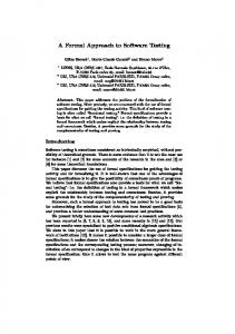
of defect-prone software entities is definitely more useful than the information about how many the software entities in question are possibly buggy. Motivation: Now take a typical application scenario as an example. Two software developers develop a new software project written in Java, and one of the developers (whose name is Jack) is responsible for software testing. Due to the tight deadline for a new release (composed of 1000+ Java classes), a sound technical solution for Jack is to identify the classes of the release that are most likely to be defect-prone before executing unit tests. Therefore, Jack builds a CPDP model based on commonly-used software metrics (such as lines of code and CK suite metrics [11]) using the Naïve Bayes (NB) classification algorithm. According to the prediction result of the CPDP model trained by other similar mature projects, only a very small percentage (about 7%) of the classes in question may be buggy, but the efficiency of the entire testing process is still relatively low because Jack has to perform random testing. In such a situation, Jack actually prefers to obtain a class ranking list that identifies the priority of each defect-prone class, so as to work out a cost-effective testing plan. Available repositories

data collection Labeled model training CPDP model defect data

(a) Construction process of a traditional CPDP model I1

test

predict CPDP model

I1 YES

I2

I2

I3

YES

NO

…

In NO

Generally speaking, WPDP has one major disadvantage that the training of WPDP models needs sufficient historical data from the same project [2]. Therefore, it is difficult to apply WPDP models to those newly created or inactive projects. With the increasing amount of labeled defect data available on the Internet, till now, CPDP has already been the most popular technique for software defect prediction, though it is still getting criticized for relatively poor prediction performance compared with WPDP [3, 4].

Figure 1. An illustration of the difference between various CPDP methods

The vast majority of prior studies on CPDP treat software defect prediction as a binary classification problem [1-8], and their main objective is to improve the prediction accuracy of CPDP models using various machine learning techniques [4, 68], such as feature selection, dimensionality reduction, and data sampling. However, estimating the defect-proneness of a given set of classes or software modules has limited effect on actual activities in software testing and software maintenance [7, 9, 10], especially when there is a lack of human resources. That is to say, from a software developer’s point of view, a ranking list

Research Objective: Unlike the studies of CPDP based on binary classification, in this paper we focus on the prediction of ranks of defect-prone software entities. An illustration of the difference between them is shown in Figure 1. In short, the main goal of this paper is to propose a ranking-oriented approach to CPDP (abbreviated as ROCPDP), which can rank buggy software entities according to priority. In addition, we also want to validate the feasibility of ROCPDP using a case study based on five open-source projects from the publiclyavailable data set AEEEM [12].

Binary classification result

I3

… In Test set

test

predict Our approach

I8 1

I2

I12

2

3

…

I1 n

Ranking prediction result (b) Comparison between traditional CPDP and our approach

DOI reference number: 10.18293/SEKE2016-047

159

at each state in future based on a defect state transition model; Rathore et al. [25] presented an approach to predicting the number of faults using Genetic Programming.

The contributions of this paper are summarized below. (1) We consider CPDP as a ranking (prediction) problem and propose a new, easy-to-use method called ROCPDP, which utilizes a simple multiple linear regression model with singleobjective optimization. Besides, we optimize the model’s parameters using the gradient descent method.

On the other hand, in recent years a few researchers tried to investigate software defect prediction from a new perspective. That is, they formulated this problem as a ranking problem rather than a binary classification problem or a regression problem [9, 21]. Therefore, the approaches to Learning to Rank (LTR) [26] in the field of information retrieval have been recently introduced to investigate software defection prediction. However, the above studies were conducted based on the assumption that the rank of a defect-prone software entity is proportional to the actual number of defects that it contains. In addition, they were also performed in WPDP scenarios using the conventional validation (e.g., partitioning the data set from a project into two sets of 80% for training and 20% for test) or 10-fold cross-validation. Hence, it is still unknown whether these methods proposed in prior studies [9, 21] can be used in practical CPDP scenarios.

(2) We conduct an empirical study based on AEEEM, and the result shows that in different CPDP scenarios our approach outperforms other benchmark methods in terms of two common evaluation metrics, i.e., Spearman’s rank correlation coefficient and Kendall rank correlation coefficient. The rest of this paper is organized as follows: Section II introduces the related work of CPDP, and Section III presents the details of our approach; in Section IV, a case study is given to demonstrate that our approach is better than the benchmark methods with regards to the given evaluation metrics; potential threats to the validity of our study are presented in Section V; in the end, Section VI summaries this paper and outlines future work directions.

III. II.

RELATED WORK

As mentioned before, CPDP is a popular defect prediction technique used to predict defects in a given project with the prediction models (also called predictors) trained based on labeled defect data from other projects [13]. After Briand et al. made an early attempt to validate the applicability of CPDP [14], many researchers in this field have tried to improve the performance of CPDP models using different techniques such as data mining and machine learning. Fortunately, recent studies have shown that it is indeed a feasible method for defect prediction in software projects with different sizes [13, 15-20]. Due to space limitations of this paper, for more details about CPDP approaches, please refer to the latest surveys [6, 7]. In these CPDP scenarios, the focus of the researches most relevant to the topic of this paper is on predicting or estimating the number of software defects/faults in a given software entity, which could be deemed as a specific problem with predictive analytics [10, 21]. In fact, this is not a new field of study. Earlier studies often trained this type of predictors using linear regression [22] or multiple regression analysis [23]. That is to say, according to training examples, these predictors were used to estimate the relationships among variables, including a dependent variable, viz. the number of defects, and one or more independent variables, viz. software metrics. More precisely, such predictors help us predict the unknown value of dependent variable from the known values of independent variables.

A RANKING-ORIENTED CPDP APPROACH

Considering the research objective of this paper, we focus on the method for predicting buggy software entities’ ranks in CPDP scenarios. Unlike previous similar studies [9, 21], we assume that the rank of a buggy software entity is proportional to the score determined by both the number of defects within the entity and the severity of each defect. The higher the score of a software entity receives, the higher its rank becomes. A. Problem Definition First of all, we build a predictor based on training examples from different software projects. Suppose that there are two ranking lists Lr and Lp for a given test set. Lr and Lp denote the actual and predicted results of defect-prone software entities, respectively, and they are partially ordered sets sorted in descending order according to the score of each software entity. So, the problem of this paper is how to minimize the difference between Lp and Lr. In other words, we want to make Lp approximate Lr as closely as possible, formally defined as max sim( L p , Lr ),

(1)

where sim is a function used to calculate the similarity between two given ranking lists. B. Description of Our Approach Inspired by the idea of the Point-wise approach to LTR [26], in this paper the above problem can be approximated by a regression problem: given the values of a set of software metrics for a software entity, predict its score. This implies that our approach is required to predict the scores of defect-prone software entities as accurately as possible. We then present the formal definition of actual/real scores as follows:

Subsequently, many other types of predictors have been built with various regression methods such as decision trees (DT), support vector regression (SVR), and Bayesian ridge regression (BRR). Moreover, our prior empirical study [10] shows that in WPDP and CPDP scenarios the DTR-based predictor is the best estimator for the number of defects among the six prediction models under discussion. To further improve the accuracy of predictions, some optimization methods have been applied to the construction of these types of predictors. For example, Wang et al. [24] applied the Discrete Time Markov Chain (DTMC) model to predict the number of defects

 k w , if the i th software entity has k bugs, ∑ j si =  j =1 0, if the i th software entity is non-defective. r

160

(2)

where w is the severity score of a bug and k is a positive integer. Note that w can be rated on a five-point or ten-point scale to score a bug’s severity.

Because the gradient descent method often takes multiple iterations to calculate a local minimum that meets the demand of accuracy, we update the value of θj in the negative direction of the gradient with a small learning rate (or known as step size) on each iteration, as defined below.

Because multiple liner regression (MLR) models have proven useful in software defect prediction [9, 27, 28], in this paper we define a simple MLR model predicting the scores of a given set of software entities, as described below. s = θ 0 + θ1 m1 + θ 2 m2 +  + θ d md =

θ j := θ j − α ⋅

d

∑θ m , i

i =0

where mi denotes the value of a given software metric, d indicates the number of software metrics, and θi is an unknown parameter of the model.

1

∑(s 2  N

− si

r

i

)

2

+λ ⋅ || θ ||

2

i =1

, 

(4)

∂L (θ ) ∂θ j (5)



∑ ( s 2

1

N

i =1



)

− si ⋅ r

i

∑

∂ ∂θ j



λ

( s − s ) + 2 ⋅ 2 ⋅ θ r

i

i



  ∂  d r s s − ⋅ ( ) ∑  i i ∂θ  ∑ θt mt − sir   + λθ j =i 1 = t 0 j   N

=

∑(s N

=m j ⋅

i =1

)

− si +λθ j . r

i

TABLE I. j

(6)

 

(7)

(

r

)

(8)

CASE STUDY

A. Data Collection The data set used in our case study is AEEEM [12], which consists of five open-source software projects written in Java and is available for free download on the Internet (website: http://bug.inf.usi.ch). Data statistics of the projects in this data set are presented in Table I. More details of the data set refer to the literature [4, 12].

∂L (θ ) ∂ 1 N λ d 2 r 2 s s = − ⋅ θj + i i ∂θ j ∂θ j  2 i 1= 2 j 0  = =2 ⋅

i =1

≈ m j ⋅ si − si +λθ j .

IV.

where the derivative with respect to any parameter θj of L(θ) is

)

)

− si +λθ j , r

i

Figure 2 displays the algorithm used for estimating the model’s parameters. Once all of the unknown parameters are fixed based on training examples, the entire learning process ends, and such a MLR model can be used for prediction. It is worth noting that evaluating the sum of gradients (see Eq. (6)) becomes very expensive if training examples are enormous. In this case, we can also utilize stochastic gradient descent to optimize the model’s parameters when dealing with very largescale data sets. That is, the gradient of θj is approximated by a gradient at a single example, thus leading to a low computation cost. Therefore, Eq. (6) can be rewritten as

C. Estimation of Model Parameters As far as we know, gradient descent is a widely used firstorder optimization algorithm. In this paper, we utilize it to find a local minimum of the above loss function, so as to estimate the unknown parameters of the model. For a given training set, the derivative with respect to θ of L(θ) is denoted as follows:

∑(

N

Figure 2. An algorithm to estimate model parameters

where θ is a vector written as (θ0, θ1, θ2, …, θd), N is the number of training examples, and λ is a small regularization parameter.

 ∂ L (θ )   ∂θ   0  ∇θ L (θ ) =   ,  ∂   L (θ )   ∂θ d 

∑(s

-----------------------------------------------------------------------------------------Algorithm 1: Estimation of Model Parameters Using Gradient Descent -----------------------------------------------------------------------------------------Input: θ, α, λ, and N training examples with d metrics and a score Output: θ 1: Initialize θ, α, and λ; 2: Randomly shuffle the training examples; 3: repeat 4: Calculate the value of s according to Eq. (3); 5: Calculate the gradient of θ according to Eq. (6); 6: Update the value of θ according to Eq. (7); 7: until convergence 8: return θ; ------------------------------------------------------------------------------------------

During the supervised learning process of a MLR model, the main goal of our method is to minimize all possible differences between values predicted by the model and the corresponding actual/real values. According to the principle of least squares, the estimation of model parameters in our method can be formulated as the minimization of a loss function, which is defined below. L (θ )=

∂θ j

 

= θ j − α ⋅ mj ⋅

where α is the learning rate (α > 0) and the symbol “:=” denotes a assignment operator.

(3)

i

∂L (θ )

Project Equinox (EQ) Eclipse JDT Core (JDT) Eclipse PDE UI (PDE) Mylyn (MYL) Apache Lucene (AL)

161

DATA STATISTICS OF AEEEM

Type # of Files % of Buggy Files # of Metrics OSGi framework 325 36.69% 71 IDE Development

997

20.66%

71

IDE Development

1492

14.01%

71

Task management Search engine library

1862

13.16%

71

399

9.26%

71

optimization algorithms (i.e., gradient descent and genetic algorithm), and the third is obtained by using LTR approaches like RankSVM [29]. The detailed introduction to the above methods/algorithms refers to subsection IV.C.

B. Experiment Design Data preprocessing. There are six types of software metrics in AEEEM, including process metrics, entropy-of-source-code metrics, entropy-of-change metrics, churn-of-source-code metrics, previous-defect metrics, and source code metrics. Because they are different in the scales of numerical values, we have to normalize the raw data from AEEEM. Although there exist many normalization methods for machine learning and data mining, prior studies [10, 13, 16, 17, 18] have proven that the normalization of training data using z-score can, to some extent, improve prediction performance of defect classification models. Hence, in this paper we apply z-score normalization to every example in AEEEM.

Performance comparison. For each project in AEEEM, we 1 can obtain four ( C5 −1 ) prediction results and one prediction result under the contexts of O2O and M2O, respectively. Such prediction results are evaluated in terms of the metrics defined in subsection IV.D. To make a reasonable comparison between our approach and the benchmark methods, we will make twenty (5×4) O2O predictions and five (5×1) M2O predictions, respectively, and then analyze their mean values of the evaluation metrics for these predictions under different CPDP contexts (see Table III).

Experiment Context Configuration. Unlike the prior studies that focus on WPDP [9, 21], in CPDP scenarios we design two types of experiment contexts, namely, one-to-one (O2O) and many-to-one (M2O). For a target project treated as a test set, the training set is a project chosen randomly from the rest of the projects in AEEEM, which is referred to as O2O. On the contrary, M2O indicates that the remaining AEEEM projects (except the target project) are used as the training set. Because some prior studies [2, 10, 13] have shown that defect prediction performs well within projects and cross projects when there is a sufficient amount of training data, in this paper we also want to examine whether our method can achieve better performance under the context of M2O. Defect Predictor Training. According to training data, three types of defect predictors are trained in the experiment contexts. The first is simply built with a few typical regression methods such as DT and SVR, the second is trained by using two classic TABLE II. Approach LR

RF

GB

DT

SVR

GA

RankSVM

RankBoost

C. Learning Methods In general, regression analysis methods are a category of quantitative methods which can predict the outcome of a given dependent variable according to the relationships with other related independent variables. In this paper, we build the first type of defect predictors with five typical regression analysis methods, namely, Linear Regression (LR), Random Forests (RF), Gradient Boosting (GB), DT, and SVR, and they are used to predict the score of each example in the test set. Due to space limitations of this paper, if readers are interested in the details of these methods, their descriptions refer to the corresponding Wikipedia entries. Note that all of the five methods are implemented with Weka [30]. Unless otherwise specified, the default parameter settings for these regression methods used in our experiments are specified by Weka.

BRIEF INTRODUCTION TO BENCHMARK APPROACHES

Brief Description Linear Regression is a widely used statistical approach to modeling the relationship between a scalar dependent variable y and one or more independent variables denoted as X, and it focuses on the conditional probability distribution of y given X. Moreover, the effectiveness of this method for predicting the number of bugs has been validated by prior studies [22, 23, 27, 28]. Random Forests, known as a notion of the general technique of random decision forests, are an ensemble learning method for regression and other tasks. For regression analysis, random forests are used by building a number of decision trees according to training data and generating an outcome that is the mean prediction of the individual decision trees, and they have been utilized as a benchmark method in [9, 10, 27]. Gradient Boosting, which is a well-known machine learning technique for regression and classification problems, combines weak prediction models into a single prediction model that has a greater capacity to deal with a given task, in a stage-wise fashion, and it often generalizes them by optimizing an arbitrary differentiable loss function. Moreover, it has been utilized as a benchmark method in [10]. Decision trees are one of the common predictive modeling approaches used in data mining and machine learning, and they are of two main types: classification tree and regression tree. When predicted results are continuous values (typically real numbers), this type of decision trees is called regression tree. Decision trees have been used as a benchmark method in [9, 10, 21, 27]. Support vector machines (SVMs) are supervised learning models that can be used for classification and regression analysis, and a version of SVM for regression is called support vector regression (SVR). The models built based on SVR require only a small subset of training data and maintain all the main features that characterize the maximum-margin algorithm. Moreover, SVR has been used as a benchmark method in [10]. An approach to predicting the number of bugs in software systems using Genetic Programming is presented in [25], and its effectiveness has been evaluated in terms of three evaluation metrics (namely, average relative error, Recall, and Completeness) for ten data sets collected from PROMISE (http://promisedata.org). RankSVM is an instance of SVM for efficiently training Ranking SVMs as defined in [29], which is used to solve certain ranking problems. In general, it belongs to one of the Pair-wise ranking methods in information retrieval field. Moreover, RankSVM has been utilized as a benchmark method in [21]. RankBoost [31] is a boosting method for ranking a given set of examples. It trains one weak learner that produces a weak ranking at each iteration, and combines these weak rankings as the final ranking function. Like all boosting algorithms, RankBoost adjusts the weights assigned to pairs of examples after each round of iteration. Moreover, RankBoost has been utilized as a benchmark method in [21].

optimization algorithms. In addition to gradient descent used in this paper, there are actually many optimization algorithms for the single-objective optimization problem, such as Genetic Algorithm (GA) and Evolutionary Programming (EP). Since

Obviously, the above defect predictors are learned without additional optimization. To improve the accuracy of CPDP predictors while maintaining their generality, we train the second type of defect predictors with typical single-objective

162

to say, the score of a class is equal to the number of bugs that it contains. Hence, all the buggy classes in AEEEM are ranked in terms of the number of bugs.

GA is the most popular type of evolutionary algorithms, we optimize this problem with GA for the purpose of comparing with the prior study [25] similar to our work. In a word, the ranks of test examples are calculated based on their scores which are predicted by the two types of defect predictors described above. Note that if two or more examples in test set get the same score, they will be sorted by example number in ascending order by default. In contrast, LTR-based defect predictors are obtained by optimizing the performance of ranking directly. In this paper, we utilize two commonly used Pair-wise approaches to LTR (i.e., RankSVM [29] and RankBoost [31]) in the field of information retrieval to train defect predictors.

TABLE III.

LR RF GB DT SVR ROCPDP GA RankSVM RankBoost

The brief introduction to these benchmark approaches used in our experiments is presented in Table II.

JDT EQ AL MYL PDE Avg.

RF S K 0.424 0.363 0.490 0.422 0.267 0.223 0.196 0.137 0.275 0.211 0.330 0.271

GB S K 0.321 0.277 0.393 0.323 0.198 0.134 0.189 0.132 0.231 0.182 0.266 0.210

Spearman M2O 0.287 (+9.96%) 0.313 (+8.68%) 0.239 (+6.22%) 0.319 (+13.93%) 0.259 (+7.02%) 0.449(+7.93%) 0.323 (+8.03%) 0.308 (+9.61%) 0.312 (+7.96%)

O2O 0.217 0.231 0.180 0.223 0.194 0.357 0.240 0.229 0.233

Kendall M2O 0.220 (+1.38%) 0.253 (+9.52%) 0.181 (+0.56%) 0.261 (+17.04%) 0.205 (+5.67%) 0.392 (+9.80%) 0.258 (+7.50%) 0.256 (+11.79%) 0.269 (+15.45%)

(1) For each of the nine approaches under discussion, the defect predictor trained under the context of M2O performs better than that trained under the context of O2O in terms of the two evaluation metrics. In particular, the defect predictor built based on DT achieves the most significant improvement of prediction performance under different CPDP contexts (as indicated by the numbers in bold in brackets). The finding, in agreement with previous studies on defect classification and regression [2, 10, 13], suggests that the prediction performance can be improved as long as there is sufficient training data collected from other projects.

E. Empirical Results Because the data set AEEEM does not actually contain the information about the severity of bugs, we have to make the assumption that the bugs in AEEEM are all identical. That is LR S K 0.437 0.385 0.513 0.441 0.222 0.167 0.252 0.198 0.291 0.226 0.342 0.283

O2O 0.261 0.288 0.225 0.280 0.242 0.416 0.299 0.281 0.289

There are two interesting findings that deserve attention, as presented in Table III.

D. Evaluation Metrics Here, we choose two widely used statistical indicators to quantify the results of defect predictors. One is the Spearman’s rank correlation coefficient (Spearman for short), which is defined as the Pearson correlation coefficient between the ranked variables; the other is the Kendall rank correlation coefficient (Kendall for short), which measures the association between two measured quantities [32]. The value of each evaluation metric ranges between -1 and 1, and higher values closer to 1 mean better prediction performance.

TABLE IV.

PREDICTION RESULTS UNDER CPDP CONTEXTS

(2) According to the two evaluation metrics, our approach, by and large, outperforms the other eight approaches under the two experiment contexts, as shown by the numbers in bold.

PERFORMANCE COMPARISON AMONG DIFFERENT METHODS DT S K 0.451 0.412 0.464 0.401 0.246 0.193 0.278 0.212 0.319 0.231 0.352 0.290

SVR S K 0.304 0.245 0.343 0.295 0.257 0.218 0.230 0.183 0.238 0.179 0.274 0.224

ROCPDP S K 0.455 0.395 0.562 0.503 0.391 0.355 0.486 0.413 0.351 0.294 0.449 0.392

GA S K 0.429 0.366 0.444 0.399 0.356 0.304 0.304 0.247 0.364 0.295 0.379 0.322

RankSVM S K 0.434 0.380 0.548 0.491 0.211 0.162 0.237 0.185 0.321 0.271 0.350 0.298

RankBoost S K 0.447 0.408 0.536 0.474 0.232 0.173 0.249 0.198 0.308 0.269 0.354 0.304

S: Spearman, K: Kendall, and the best result determined by both the two evaluation metrics is highlighted in bold type.

is, on average, better than the other eight approaches performed in the WPDP scenario in terms of both the two evaluation metrics. Compared with these benchmark methods, the performance improvements with respect to Spearman range from 18.47% (on GA) to 68.80% (on GB), and they span from 21.74% (on GA) to 86.67% (on GB) in terms of Kendall. Generally speaking, according to the results of Tables III and IV, under the context of M2O our method outstrips the benchmark methods conducted in both CPDP and WPDP scenarios, which suggests that it can be applied to those projects with very little historical defect data.

Because our prior study [10] has shown that CPDP models for bug numbers are comparable to (or sometimes better than) those WPDP models with respect to prediction performance. That is, there are actually no significantly statistical differences between the two types of defect predictors. To further validate the effectiveness of our method, we compared our method performed under the context of M2O with the benchmark approaches conducted in WPDP scenarios. We trained eight new defect predictors in a specific WPDP scenario that has been used in [21]. For each target project in Table IV (see the first column), we randomly selected 80% of class files of the project as training data, and the remainder of the files was used as test data. We repeated this step 20 times and used the average of prediction results for the 20 executions as the final result. As shown in Table IV, because our method obtains the best result three times under the context of M2O, it

V.

THREATS TO VALIDITY

The most interesting result of this paper is that the defect predictor built with our method under the context of M2O is, on average, better than those trained by using different types

163

[7]

of typical learning methods in both CPDP and WPDP scenarios. Even so, there are still some potential threats to the validity of our work, one of which concerns the generalization of the finding. The reasons mainly lie in the following aspects: 1) only the 5 projects in AEEEM is used in our experiments, implying that we need to validate the general effectiveness of our method on larger data sets from real-world software projects; 2) because the information about the severity of bugs is missing in AEEEM, we have to rank all the examples in question in terms of the number of bugs instead of its actual score; 3) in the WPDP and CPDP scenarios, we select training data in a simple way, though there are many time-consuming but effective methods for feature selection and dimension reduction [21]; and 4) we only utilize eight typical methods that belong to three different categories, namely, regression analysis, single-objective optimization, and learning to rank, without additional optimization for a given data set. VI.

[8]

[9]

[10] [11] [12] [13]

[14]

CONCLUSION AND FUTURE WORK [15]

In recent years CPDP has become very popular in software engineering, but it is often treated as a binary classification or regression problem in most of prior studies. To facilitate actual development activities in projects with limited manpower and time, in this paper we consider it as a ranking problem and propose a ranking-oriented CPDP method. Interestingly, the empirical results obtained based on AEEEM show that the defect predictor built with our method under the context of M2O is, on average, better than those trained by using the benchmark methods in both CPDP and WPDP scenarios. This suggests that our method is a sound choice to train defect predictors for those newly created or inactive software projects.

[16]

[17]

[18] [19] [20]

As an initial attempt to construct ranking-oriented defect predictors in different CPDP scenarios, the proposed approach in this paper needs to be improved. So, our future work is to accurately predict the Top-k ranking for buggy software entities.

[21]

[22] [23]

ACKNOWLEDGEMENT This work is supported by the 973 Program of China (No. 2014CB340404) and the National Natural Science Foundation of China (Nos. 61272111 and 61273216).

[24]

REFERENCES

[26]

[1] [2]

[3]

[4]

[5]

[6]

[25]

C. Catal, “Software fault prediction: a literature review and current trends,” Expert Systems with Applications, 2011, 38 (4): 4626–4636. T. Zimmermann, N. Nagappan, H. Gall, E. Giger, and B. Murphy, “Cross-project defect prediction: a large scale experiment on data vs. domain vs. process,” in: ACM Proc. of ESEC/FSE 2009, pp. 91–100. T. Hall, S. Beecham, D. Bowes, D. Gray, and S. Counsell, “A systematic review of fault prediction performance in software engineering,” IEEE Transactions on Software Engineering, 2012, 38 (6): 1276–1304. M. D’Ambros, M. Lanza, and R. Robbes, “Evaluating defect prediction approaches: a benchmark and an extensive comparison,” Empirical Software Engineering, 2012, 17(4-5): 531–577. D. Radjenović, M. Heričko, R. Torkar, and A. Živkovič, “Software fault prediction metrics: A systematic literature review,” Information and Software Technology, 2013, 55(8): 1397-1418. G. Abaei and A. Selamat, “A survey on software fault detection based on different prediction approaches,” Vietnam Journal of Computer Science, 2014, 1(2): 79-95.

[27]

[28]

[29] [30]

[31]

[32]

164

R. Malhotra, “A systematic review of machine learning techniques for software fault prediction,” Applied Soft Computing, 2015, 27: 504–518. H.J. Wang, T.M. Khoshgoftaar, and Q.A. Liang, “A study of software metric selection techniques: stability analysis and defect prediction model performance,” International Journal on Artificial Intelligence Tools, 2013, 22(5): 1360010. X. Yang, K. Tang, and X. Yao, “A Learning-to-Rank Approach to Software Defect Prediction,” IEEE Transactions on Reliability, 2015, 64(1): 234-246. M.M. Chen and Y.T. Ma, “An empirical study on predicting defect numbers,” in: Proc. of SEKE 2015, USA, 2015, pp. 397-402. S.R. Chidamber and C.F. Kemerer, “A metrics suite for object oriented design,” IEEE Trans. on Software Engineering, 1994, 20(6): 476-493. M. D’Ambros, M. Lanza, and R. Robbes, “An extensive comparison of bug prediction approaches,” in: IEEE Proc. of MSR 2010, pp. 31-41. P. He, B. Li, X. Liu, J. Chen, and Y.T. Ma, “An empirical study on software defect prediction with a simplified metric set,” Information and Software Technology, 2015, 59: 170–190. L.C. Briand, W.L. Melo, and J. Wüst, “Assessing the applicability of fault-proneness models across object-oriented software projects,” IEEE Transactions on Software Engineering, 2002, 28(7): 706–720. J. Nam, S.J. Pany, and S. Kim, “Transfer Defect Learning,” in: IEEE/ACM Proc. of ICSE 2013, USA, 2013, pp. 382–391. B. Turhan, A.T. Misirli, and A. Bener, “Empirical evaluation of the effects of mixed project data on learning defect predictors,” Information and Software Technology, 2013, 55(6): 1101–1118. Z. He, F. Shu, Y. Yang, M.S. Li, and Q. Wang, “An investigation on the feasibility of cross-project defect prediction,” Automated Software Engineering, 2012, 19(2): 167–199. F. Peters, T. Menzies, and A. Marcus, “Better cross company defect prediction,” in: IEEE Proc. of MSR 2013, USA, 2013, pp. 409-418. S. Herbold, “Training data selection for cross-project defect prediction,” in: ACM Proc. of PROMISE 2013, USA, 2013, p. 6. F. Rahman, D. Posnett, and P. Devanbu, “Recalling the imprecision of cross-project defect prediction,” in: ACM Proc. of FSE 2012, p. 61. T.T. Nguyen, T.Q. An, V.T. Hai, and T.M. Phuong, “Similarity-based and rank-based defect prediction,” in: IEEE Proc. of ATC 2014, pp. 321-325. J.E. Gaffney Jr., “Estimating the Number of Faults in Code,” IEEE Transactions on Software Engineering, 1984, 10(4): 459-465. N.E. Fenton and M. Neil, “A Critique of Software Defect Prediction Models,” IEEE Trans. on Software Engineering, 1999, 25(5): 675-689. J. Wang and H. Zhang, “Predicting defect numbers based on defect state transition models,” in: ACM Proc. of ESEM 2012, pp. 191-200. S.S. Rathore and S. Kumar, “Predicting Number of Faults in Software System using Genetic Programming,” Procedia Computer Science, 2015, 62: 303–311. T.-Y. Liu, “Learning to Rank for Information Retrieval,” Foundations and Trends in Information Retrieval, 2009, 3(3): 225–331. E.J. Weyuker, T.J. Ostrand, and R.M. Bell, “Comparing the effectiveness of several modeling methods for fault prediction,” Empirical Software Engineering, 2010, 15(3): 277–295. K. Gao and T. M. Khoshgoftaar, “A comprehensive empirical study of count models for software defect prediction,” IEEE Transactions on Reliability, 2007, 56(2): 223–236. T. Joachims, “Optimizing search engines using clickthrough data,” in: ACM Proc. of KDD 2002, Canada, 2012, pp. 133–142. M. Hall, E. Frank, G. Holmes, B. Pfahringer, P. Reutemann, and I.H. Witten, “The WEKA Data Mining Software: An Update,” SIGKDD Explorations, 2009, 11(1): 10–18. Y. Freund, R. Iyer, R. Schapire, and Y. Singer, “An efficient boosting algorithm for combining preferences,” Journal of Machine Learning Research, 2003, 4: 933–969. M. Kendall, “A New Measure of Rank Correlation,” Biometrika, 1938, 30(1–2): 81–89.