A Realistic Framework for Delay-Tolerant Network Routing in ... - MIT

A Realistic Framework for Delay-Tolerant Network Routing in Open Terrains with Continuous Churn Veeramani Mahendran, Sivaraman K. Anirudh, and C. Siva Ram Murthy Department of Computer Science and Engineering Indian Institute of Technology Madras Chennai-600036, India

Abstract. The conventional analysis of Delay-Tolerant Network (DTN) routing assumes that the terrain over which nodes move is closed implying that when the nodes hit a boundary, they either wrap around or get reflected. In this work, we study the effect of relaxing this closed terrain assumption on the routing performance, where a continuous stream of nodes enter the terrain and get absorbed upon hitting the boundary. We introduce a realistic framework that models the open terrain as a queue and compares performance with the closed terrain for a variety of routing protocols. With three different mobility scenarios and four different routing protocols, our simulation shows that the routing delays in an open terrain are statistically equivalent to those in closed terrains for all routing protocols. However, in terms of cost some protocols differ widely in two cases while some continue to demonstrate the statistical equivalence. We believe that this could be a new way to classify routing protocols based on the difference in their behavior under churn. Keywords: Delay-tolerant network, routing, mobility model, open terrain.

1

Introduction

Delay-Tolerant Networks (DTNs) are a class of networks that are characterized by intermittent connections, long variable delays, and heterogeneous operating environments over which an overlay or bundle layer works [5,6,7]. DTNs find potential applications in many areas such as satellite networks, vehicular networks, and disaster response systems. Routing protocols in DTN work on the basis of the store, carry, and forward paradigm [5], where a node carries the message until it encounters the destination node or any other node that has high probability of meeting the destination node. Based on this paradigm various DTN routing protocols have been proposed. Naive approaches such as epidemic routing [16] amount to flooding the network with copies of the message and more sophisticated approaches such as utility based routing [12,15] forward the message to the encountered node that is found M.K. Aguilera et al. (Eds.): ICDCN 2011, LNCS 6522, pp. 407–417, 2011. c Springer-Verlag Berlin Heidelberg 2011

408

V. Mahendran et al.

to be a good message-carrier (based on heuristic estimates) for the destination node. DTN routing protocols are not constrained by the closed terrain assumption, however, the theoretical analysis and simulation based results [8, 14] are marked by the fundamental assumption that the terrain over which the nodes move is closed, i.e., they make one of the two assumptions: nodes either wrap around or are reflected at the terrain boundaries. For instance, one of the best performing protocols in this class ‘spray-n-wait’ routing protocol [13] computes the total number of copies to spray from a system of recursive equations that assume the number of node infections at any time as a monotonically increasing function bounded by the total number of nodes. In this work, we look at the performance analysis of DTN routing protocols when the assumption of closed terrain is relaxed. In particular, we assume that once the node reaches the boundary of the simulation area, it is “absorbed” and hence no longer participates in routing since it is effectively out of range. This situation simulates a realistic scenario where nodes that move past a particular boundary of a region such as a stadium or an open air theater are very likely to move out through one of the exits. The physical obstacles such as the boundary wall disable the nodes from participating in routing once they cross a boundary. We also explicitly model churn in the network, by having these nodes enter the terrain as a Poisson process and exit by hitting one of the boundaries. In summary, the contributions of this paper are threefold: 1. We introduce a novel and realistic open terrain framework that explicitly models the influx and outflux of nodes in the terrain. This framework also provides a way to compare the open and closed terrains in terms of their routing performance. 2. We simulate a variety of routing protocols under different mobility scenarios using the above framework. We conclude that the open terrains are statistically equivalent to the closed ones in terms of routing delay. 3. We also observe that some protocols exhibit the statistical equivalence in terms of send cost, however, some do not. This could potentially provide us a new way to classify routing protocols. The structure of the rest of this paper is outlined as follows: Section 2 presents the related work in this area. Section 3 describes the framework for studying open terrains. Section 4 explains the simulation setup for the experiments using the new framework. In Section 5, we interpret the simulation results and explain their trends. We conclude our work in Sect. 6 and describe some future directions in Sect. 7.

2

Related Work

Open terrains have been considered in the analysis of cellular networks where users dynamically enter and leave hexagonal cells according to some mobility model. The time spent by the users in the range of a tower (serving any one

A Realistic Framework for Delay-Tolerant Network Routing

409

cell), or the time spent by the users in the overlapping region of two towers is considered as an important derived attribute for that mobility model. The distribution of these times is useful in designing appropriate hand-off schemes for cellular networks [9]. However, the scenario considered there is starkly different since the towers serve as an infrastructure linked by cables forming a stable wired backbone for communication. On the other hand, we model a completely opportunistic and cooperative routing where there is no infrastructure support. The work that is closest to ours in terms of being applicable to a DTN is the work on modeling Pedestrian Content Distribution on a network of roads [17]. Every street segment is modeled as an M/G/∞ queue, where every node picks a speed from the entry point to the exit point on the street that is uniformly distributed in a range [vmin , vmax ]. The road network is treated as a network of such queues. However, the scenario we consider here is routing and not content dissemination. Additionally, the mobility on the street is one dimensional.

3

A Framework for Studying Open Terrains with Continuous Churn

In this section, we describe the framework to model open terrain as a queue that enables it to have a fair comparison with the closed terrain in studying their routing performance. 3.1

Terrain Model

In our framework, the node enters a square terrain at some point on the boundary, the point being chosen uniformly over the perimeter of the terrain. The node continues to move, according to some mobility model, until it hits one of the boundaries where it is absorbed. The essential difference between a closed terrain and an open terrain under this framework is: 1. When a node hits the boundary it either reflects or wraps around in case of a closed terrain, but is merely absorbed and dies in the case of an open terrain. 2. The continuous churn implies that there will at any time, be an influx of nodes into the terrain and an outflux of nodes getting absorbed. The influx process is described in the next section. We believe this model of an open terrain to be realistic since it represents many day-to-day scenarios, where nodes that move towards the boundary of an enclosed space such as a theater are likely to move out through an exit. Beyond that, the boundaries render any peer-to-peer communication between nodes impossible. 3.2

Open Terrains as Queues

The nodes are assumed to arrive as a Poisson process. This Markovian arrival process models continuous churn too. Thus the terrain taken as one system

410

V. Mahendran et al.

behaves like an infinite server queue with a Markovian arrival process and a service time given by a general distribution. So, in the Kendall notation it is an M/G/∞ queue. Continuing with this queuing model, the sojourn time E(t) of a node is the time it stays inside the terrain boundaries. 3.3

Equalizing the Open and Closed Terrains

This framework would not be complete unless there was a way to compare the open and closed terrains for any given application. We “equalize” the two terrains as follows: 1. Let N be the total number of nodes in the closed terrain. 2. The expected sojourn time or service time E[t] of the open terrain is computed as a function of the dimensions of the terrain and the mobility model of the nodes inside the terrain. E[t] = f (T errain dimension, M obility model)

(1)

This can also be computed empirically via simulations (as we have done in this work). 3. Little’s Law is applied to determine the arrival rate λ such that the average number of nodes in the open terrain E[n] is same as the total number of nodes N , thereby equalizing with that of the closed terrain. λ =

E[n] E[t]

(2)

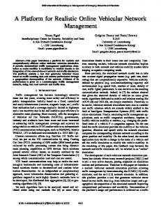
Note that the arrival rate in closed terrain case is immaterial since the simulation in the closed terrain starts only once all nodes are inside. The equality of the open and closed terrains as per the above procedure is shown in Fig. 1 for three different mobility models. The straight line at 100 represents the number of nodes in the closed terrain. 120

120

MIT

100

80 60 40

80 60 40

20

20

0

0

0

200

400

600

800

Time (seconds)

1000

(a) MIT Trace

1200

RW

100

Number of nodes

Number of nodes

100

Number of nodes

120

VANET

80 60 40 20

0

200

400

600

800

1000

1200

0

0

200

400

(b) VANET Trace

600

800

1000

1200

Time (seconds)

Time (seconds)

(c) RWMM Trace

Fig. 1. Variation of number of nodes versus time

1400


4

411

Simulation Setup

We used a well known discrete event network simulator ns-2 [1] to simulate various routing protocols under the open and closed terrain scenarios using the framework described in Section 3. The simulation parameters are shown in Table 1. We have not considered any traffic model as such, since the goal was to study the propagation of a single message through the open terrain and the closed terrain. Table 1. Simulation parameters Parameter Value Number of nodes 50 − 250 Buffer size ∞ Velocity of nodes ‘V ’ 5m/s Terrain size 1000m × 1000m MAC protocol IEEE 802.11 Transmission range 20m Carrier sense range 40m Number of simulation runs 100 Total simulation time 1000s

4.1

Routing Protocols

The four routing protocols used for simulation are described below: 1. Epidemic routing: In this scheme [16], every node forwards the message to every other node it encounters and due to this it is optimal in terms of delay, but at the expense of very high cost1 . To preserve the common denominator across the routing protocols under test, no explicit recovery mechanisms are considered to stop the replication. Rather, we have considered the costs and delay incurred only till the message reaches the destination node. 2. Two-hop routing: The source node forwards the message to either the relay node or the destination node and the relay nodes in turn forward the message only to the destination node. 3. Spray-n-wait routing: Here, as described in [13] a fixed number of copies of the message, say L, is handed over to the source node, which in turn hands over half the message copies to any node it encounters until the source node runs out of message copies (Binary spray). Every node in turn that receives the message copies, does the same thing: i.e., if it has say x copies and encounters a node that has no copies, it hands over x/2 copies to that node and keeps the rest with itself. This process continues for any node until that node has only one copy of the message left with itself, in which case it switches to the second phase of the routing: Waiting. In this phase, the node that has only one copy of the message waits until it comes into direct contact with the destination node. 1

Cost in this context is the message passing overhead.

412

V. Mahendran et al.

4. Direct transmission: In this scheme the source node just waits until it comes into contact with the destination node and transmits only then. It has the minimum cost, but consequently has the smallest delivery ratio and largest delivery delay. 4.2

Mobility of Nodes

We use two forms of mobility models for our simulations as described below: 1. Random Walk Mobility Model (RWMM): In this model, the nodes are assumed to move at a constant speed V , throughout the simulation duration with no pause time. The choice of speed only affects the scaling of the time required for the simulation. On every epoch the node chooses a flight from an exponentially distributed random variable of a given mean. This mean is a scaled down version of the terrain side (assuming a square terrain). Next, the node picks a direction from the uniform distribution with values between [0, 2π] and then executes a flight in that direction. Once that flight terminates, the node repeats the same process over again until one of the flights takes the node to the terrain boundary in the open case where it simply gets absorbed. We use a variant of the mobility model described in [4] and modify the code provided at [3] for this purpose. 2. Time Variant Community Model (TVCM): In this model [11], the terrain is divided into many sub terrains each of which is called a community. At every point in time, a given node can be in any one of the communities. Nodes move from one community to another (at a fixed global velocity V ) using transition probabilities, akin to a Markov Chain. This whole structure of communities and their associated transition probabilities remains fixed for one time period of some duration. The node executes a sequence of different time periods and then comes back to its original starting time period again. Every node can have an independent TVCM model for itself or like the vanilla models they can be iid. The essential components that this model captures are skewed location preferences (people like to stick to their home or office) and recurrent behavior of human mobility (i.e., one community structure for the time during the weekday, one for the time during weeknights, one for weekend mornings, one for weekend nights, and so on. Also observe that the same thing would repeat itself every week). An open terrain is modeled in this case by assuming that if an epoch falls out of the boundary of the terrain it has been absorbed. If on the other hand it merely falls outside the boundary of the current community, it is reflected as in the closed terrain case. This model has the advantage of being more realistic and has been shown to successfully capture real world traces through an appropriate choice of parameters in the model. We use two types of real world models to generate traces. One is representative of VANETs and is implemented in [10]. The second model is used to generate traces based on parameters derived by matching the TVCM model to the trace observed in [2]. We use the TVCM model to simulate the two traces just cited, and will call the traces MIT and VANET henceforth for the purpose of discussion.


413

As mentioned above, we use three mobility models: a vanilla RWMM model and two models based on TVCM called MIT and VANET. 4.3

Handling Transients

Particular care must be taken to ensure that the simulation in the open terrain case is carried out only over the stationary2 phase. The simulation plot in Fig. 1 shows how the number of nodes in the terrain builds up to a particular point and then oscillates around a mean for the most part. The relatively oscillatory phase corresponds to the stationary phase and the average value around that time is the average number of nodes in the simulation area in the open case. To take care of transients, we use the mean sojourn time of that particular terrain which can be found by running the mobility model over a large set of nodes (10000 in our case) and empirically computing the mean. The mean sojourn time is large enough for the queue to stabilize to the average value. The empirical estimation is required as mentioned earlier in the framework to equalize the two terrains. Once the transient time has passed, the source begins transmitting its message. 4.4

Handling the Source and the Destination

Since we intend to compare the delivery delay between the open terrain and the closed terrain, we must ensure that with enough simulation time the message must be delivered from the source to the destination with high probability. To guarantee this, the source and destination are treated in the open terrain as “closed” terrain nodes so that there is little chance that either of them wanders off. Our work focuses on the effect of open terrains on intermediate relay nodes and we seek to avoid the premature termination of messages because of the absence of source or destination nodes in the terrain. 4.5

Performance Metrics

1. Delivery ratio: The average fraction of message transmissions that actually reach the destination. 2. Delivery delay: The average time taken to send a message from the source node to the destination node. 3. Send cost: Average number of message copies sent by all the nodes for sending a message from the source node to the destination node.

5

Simulation Results

The four routing protocols epidemic routing, two-hop routing, direct transmission, and spray-n-wait routing were simulated over 100 runs for each of the 2

Stationary in this context is the period of time the average number of nodes in the terrain remains essentially constant and same as the closed terrain.

414

V. Mahendran et al.

60

80

Send cost (messages)


SnW-Open Direct-Closed

40

Direct-Open 30 20 10

60

SnW-Closed

50

SnW-Open Direct-Closed

40

Direct-Open

30 20 10

30 20 10 0

-10

-10

150

200

250

50

100

150

200

Direct-Open

40

-10 Number of nodes

Direct-Closed

50

0 100

SnW-Open

60

0

50

SnW-Closed

70 Send cost (messages)

SnW-Closed 50

250

50

100

Number of nodes

(a) MIT trace

150

200

250

Number of nodes

(b) VANET trace

(c) RWMM trace

Fig. 2. Send cost for spray-n-wait and direct transmission 400 SnW-Closed

300

Direct-Closed

250

Direct-Open

200 150 100 50

1000

SnW-Closed

350

SnW-Open

Delivery delay (seconds)


350

SnW-Open

300

Direct-Closed

250

Direct-Open


400

200 150 100 50

0

SnW-Open 800

100

150

200

250

Direct-Closed Direct-Open

600 400 200

0 50

SnW-Closed

0 50

100

Number of nodes

150

200

250

50

100

Number of nodes

(a) MIT trace

150

200

250

Number of nodes

(b) VANET trace

(c) RWMM trace

Fig. 3. Routing delay for spray-n-wait and direct transmission

900 800

ER-Closed

ER-Open

700

ER-Open

600

2Hop-Closed

2Hop-Closed 2Hop-Open

300 200 100

500

800 Send cost (messages)

400

ER-Closed Send cost (messages)


500

2Hop-Open

400 300 200 100

0 100

150

200

Number of nodes

(a) MIT trace

250

600

ER-Closed ER-Open 2Hop-Closed 2Hop-Open

500 400 300 200 100

0 50

700

0 50

100

150

200

Number of nodes

(b) VANET trace

250

50

100

150

200

250

Number of nodes

(c) RWMM trace

Fig. 4. Send cost epidemic routing and two-hop routing

following traces, (i) VANET profile for the TVCM, (ii) MIT profile for the TVCM, and (iii) Vanilla RWMM model. All performance metrics are plotted with 95% confidence. In order to verify our framework, we pick a mobility trace for each of the models at random and plot the evolution of the number of nodes inside the


415

140

ER-Closed

120

ER-Open

120

ER-Open

2Hop-Closed

100

2Hop-Open 80 60 40 20 0

2Hop-Closed

100

2Hop-Open 80 60 40 20

100

150

200

Number of nodes

(a) MIT trace

250

ER-Open

600

2Hop-Closed

500

2Hop-Open

400 300 200 100

0 50

ER-Closed

700 Delivery delay (seconds)

ER-Closed Delivery delay (seconds)


800 140

0 50

100

150

200

Number of nodes

(b) VANET trace

250

50

100

150

200

250

Number of nodes

(c) RWMM trace

Fig. 5. Routing delay for epidemic routing and two-hop routing

terrain with time. The relatively stable part corresponds to the stationary phase of the queue. As seen in Fig. 1, the average number in the open case, is more or less the same as the number of nodes as in the closed terrain case. We depict performance in terms of two metrics i.e., delivery delay and send cost. The delivery ratio was also computed across all the protocols, but since it was close to one in all cases except direct transmission, we choose not to include those plots due to space constraints. The direct transmission protocol depends only on the source and destination nodes for the delivery of packets and hence as expected, Fig. 2 and Fig. 3 show no difference in terms of any of the metrics between the two terrains, since the source and the destination are still “closed” nodes. Figure 2 shows very little difference in send cost between the two terrains when the protocol used is either spray-n-wait or direct transmission. The only place where a little discernible, but not so vast difference shows up is the VANET trace. The same statistical equivalence in terms of the send cost of routing seems to hold for two-hop transmission too as seen in the Fig. 4. However, the epidemic routing in Fig. 4 shows the vast difference between the two mobility scenarios that gets more and more pronounced as the number of nodes increases. For instance, in the MIT trace the epidemic routing cost difference between the open and closed terrain is a factor of 2 with 50 nodes but increases to a factor of 3 when the number of nodes is 250. A similar trend seems to hold for the other two mobility traces as well, where the epidemic routing cost in an open terrain is between 3 to 4 times that of the closed terrain. This is primarily because epidemic routing does not replicate if the other node already has a copy of the message thereby saving a lot more in the case of closed terrains than in the open terrain case. Most probably this property should hold for any probabilistic version of epidemic routing as well. We expect that the difference between the open and closed cases would be significant when the probability of forwarding is high. This allows us the interesting possibility of classifying various routing protocols based on whether or not they show a difference in routing cost.

416

V. Mahendran et al.

As seen in the Fig. 3 and Fig. 5, there is little or no statistical difference in terms of the routing delay between the open and the closed terrains, which allows us to conclude that they are statistically equivalent.

6

Conclusions

This work proposed a novel and realistic framework that explicitly represents open terrains in a DTN and exhaustively compares the open and closed terrains in terms of delivery ratio, routing delay, and send cost across a range of mobility models and routing protocols. We conclude that, for all protocols, the routing delay lie in roughly the same range. Hence as far as routing delay is concerned, the open and closed terrains are statistically equivalent. The significant increase (3 to 4 times) in terms of send cost for epidemic routing in an open terrain points to the possibility of designing an intelligent routing protocol, depending on the likelihood of a node moving out and also provides a way of classifying the routing protocols based on the statistical equivalence in their performance across the open and closed terrains.

7

Future Work

The expected service time E[t] for a given simulation configuration is determined empirically by plotting the service times observed over a large ensemble of entering and subsequently exiting nodes. Future work would extend the computation of sojourn time distribution E[t] analytically. This work considers the fact that all nodes that hit the boundary gets absorbed. Future work would also consider the scenario in which a fraction of nodes that move out of the terrain are injected back. This would allow us to study the performance with a mixture of nodes.

References 1. The Network Simulator, http://www.isi.edu/nsnam/ns 2. Balazinska, M., Castro, P.: Characterizing Mobility and Network Usage in a Corporate Wireless Local-Area Network. In: MobiSys 2003: Proceedings of the 1st International Conference on Mobile systems, Applications, and Services, pp. 303– 316 (2003) 3. Camp, T.: Toilers (2002), http://toilers.mines.edu/Public/CodeList 4. Camp, T., Boleng, J., Davies, V.: A Survey of Mobility Models for Ad hoc Network Research. Wireless Communications and Mobile Computing: Special Issue on Mobile Ad hoc Networking: Research, Trends, and Applications 2(5), 483–502 (2002) 5. Cerf, V., Burleigh, S., Hooke, A., Torgerson, L., Durst, R., Scott, K., Fall, K., Weiss, H.: RFC 4838, Delay-Tolerant Networking Architecture. IRTF DTN Research Group (2007)


417

6. Fall, K.: A Delay-Tolerant Network Architecture for Challenged Internets. In: SIGCOMM 2003: Proceedings of the Conference on Applications, Technologies, Architectures, and Protocols for Computer Communications, pp. 27–34 (2003) 7. Fall, K.R., Farrell, S.: DTN: An Architectural Retrospective. IEEE Journal on Selected Areas in Communications 26(5), 828–836 (2008) 8. Garetto, M., Leonardi, E.: Analysis of Random Mobility Models with PDE’s. In: MobiHoc 2006: Proceedings of the 7th ACM International Symposium on Mobile Ad hoc Networking and Computing, pp. 73–84 (2006) 9. Hong, D., Rappaport, S.: Traffic Model and Performance Analysis for Cellular Mobile Radio Telephone Systems with Prioritized and Nonprioritized Handoff Procedures. IEEE Transactions on Vehicular Technology 35(3), 77–92 (1986) 10. Hsu, W.: Time Variant Community Mobility Model (2007), http://nile.cise.ufl.edu/~ weijenhs/TVC_model 11. Hsu, W., Spyropoulos, T., Psounis, K., Helmy, A.: Modeling Time-Variant User Mobility in Wireless Mobile Networks. In: INFOCOM 2007: Proceedings of the 26th IEEE International Conference on Computer Communications, pp. 758–766 (2007) 12. Ip, Y.K., Lau, W.C., Yue, O.C.: Performance Modeling of Epidemic Routing with Heterogeneous Node Types. In: ICC 2008: Proceedings of the IEEE International Conference on Communications, pp. 219–224 (2008) 13. Spyropoulos, T., Psounis, K., Raghavendra, C.S.: Spray and Wait: An Efficient Routing Scheme for Intermittently Connected Mobile Networks. In: WDTN 2005: Proceedings of the ACM SIGCOMM Workshop on Delay-Tolerant Networking, pp. 252–259 (2005) 14. Spyropoulos, T., Psounis, K., Raghavendra, C.S.: Performance Analysis of Mobility-Assisted Routing. In: MobiHoc 2006: Proceedings of the 7th ACM International Symposium on Mobile Ad hoc Networking and Computing, pp. 49–60 (2006) 15. Spyropoulos, T., Turletti, T., Obraczka, K.: Routing in Delay-Tolerant Networks Comprising Heterogeneous Node Populations. IEEE Transactions on Mobile Computing 8(8), 1132–1147 (2009) 16. Vahdat, A., Becker, D.: Epidemic Routing for Partially Connected Ad hoc Networks. Tech. Rep. CS-2000-06, Duke University (2000) 17. Vukadinović, V., Helgason, O.R., Karlsson, G.: A Mobility Model for Pedestrian Content Distribution. In: SIMUTools 2009: Proceedings of the 2nd International Conference on Simulation Tools and Techniques, pp. 1–8 (2009)