A Recurrent Graph Neural Network for Multi-Relational Data

A RECURRENT GRAPH NEURAL NETWORK FOR MULTI-RELATIONAL DATA Vassilis N. Ioanndis?

arXiv:1811.02061v1 [cs.LG] 5 Nov 2018

?

Antonio G. Marques†

Georgios B. Giannakis?

Digital Technology Center and Dept. of ECE, University of Minnesota, Minneapolis, USA † Dept. of Signal Theory and Comms., King Juan Carlos University, Madrid, Spain

ABSTRACT The era of “data deluge” has sparked the interest in graph-based learning methods in a number of disciplines such as sociology, biology, neuroscience, or engineering. In this paper, we introduce a graph recurrent neural network (GRNN) for scalable semisupervised learning from multi-relational data. Key aspects of the novel GRNN architecture are the use of multi-relational graphs, the dynamic adaptation to the different relations via learnable weights, and the consideration of graph-based regularizers to promote smoothness and alleviate over-parametrization. Our ultimate goal is to design a powerful learning architecture able to: discover complex and highly non-linear data associations, combine (and select) multiple types of relations, and scale gracefully with respect to the size of the graph. Numerical tests with real data sets corroborate the design goals and illustrate the performance gains relative to competing alternatives. Index Terms— Deep neural networks, graph recurrent neural networks, graph signals, multi-relational graphs. 1. INTRODUCTION A task of major importance in the interplay between machine learning and network science is semi-supervised learning (SSL) over graphs. In a nutshell, SSL aims at predicting or extrapolating nodal attributes given: i) the values of those attributes at a subset of nodes and (possibly) ii) additional features at all nodes. A relevant example is protein-to-protein interaction networks, where the proteins (nodes) are associated with specific biological functions, thereby facilitating the understanding of pathogenic and physiological mechanisms. While significant progress has been achieved for this problem, most works consider that the relation among the nodal variables is represented by a single graph. This may be inadequate in many contemporary applications, where nodes may engage on multiple types of relations [1], motivating the generalization of traditional SSL approaches for single-relational graphs to multi-relational graphs1 . In the particular case of social networks, each layer of the graph could capture a specific form of social interaction, such as friendship, family bonds, or coworker-ties [2]. Albeit their ubiquitous presence, development of SSL methods that account for multi-relational networks is only in its infancy, see, e.g., [1, 3]. Related work. A popular approach for graph-based SSL methods is to assume that the true labels are “smooth” with respect to the underlying network structure, which then motivates leveraging the topology of the network to propagate the labels and increase classification performance. Graph-induced smoothness may be captured The work in this paper has been supported by USA NSF grants 171141, 1500713, and 1442686, and by the Spanish grants MINECO KLINILYCS (TEC2016-75361-R) and Instituto de Salud Carlos III DTS17/00158. 1 Many works in the literature refer to these graphs as multi-layer graphs.

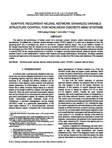
by kernels on graphs [4, 5]; Gaussian random fields [6]; or low-rank parametric models based on the eigenvectors of the graph Laplacian or adjacency matrices [7, 8]. Alternative approaches use the graph to embed the nodes in a vector space, and classify the points [9–11]. More recently, another line of works postulates that the mapping between the input data and the labels is given by a neural network (NN) architecture that incorporates the structure of the graph [12–14]. The parameters describing the NN are then learned using labeled examples and feature vectors, and those parameters are finally used to predict the labels of the unobserved nodes. See, e.g., [14], for stateof-the-art results in SSL using a single-relational graph when nodes are accompanied with additional features. Contributions. This paper develops a deep learning framework for SSL over multi-relational data. The main contributions are i) we postulate a (tensor-based) NN architecture that accounts for multirelational graphs, ii) we define mixing coefficients that capture how the different relations affect the desired output and allow those to be learned from the examples, which enables identifying the underlying structure of the data; iii) at every layer we propose a recurrent feed of the data that broadens the class of (graph signal) transformations the NN implements and facilitates the diffusion of the features across the graph; and iv) in the training phase we consider suitable (graphbased) regularizers that avoid overfitting and further capitalize on the topology of the data. 2. MODELING AND PROBLEM FORMULATION Consider a network of N nodes, with vertex set V := {v1 , . . . , vN }, connected through I relations. The connectivity at the i-th relation is captured by the N × N matrix Si , and the scalar Snn0 i represents the influence of vn to vn0 under the i-th relation. In social networks for example, these may represent the multiple types of connectivity among people such as Facebook, LinkedIn, and Twitter; see Fig.1. The matrices {Si }Ii=1 are collected in the N × N × I tensor S. The graph-induced neighborhood of vn for the i-th relation is Nn(i) := {n0 : Snn0 i 6= 0, vn0 ∈ V}.

(1)

We associate an F ×1 feature vector xn to the n-th node, and collect > > those vectors in the N ×F feature matrix X := [x> 1 , . . . , xN ] . The entry Xnp may denote, for example, the salary of the n-th individual in the LinkedIn social network. We also consider that each node n has a label of interest yn ∈ {0, . . . , K − 1}, which may represent, for example, the education level of a person. In SSL we have access to the labels only at a subset of nodes {yn }n∈L , with L ⊂ V. This partial availability may be attributed to privacy concerns (medical data); energy considerations (sensor networks); or unrated items (recommender systems). The N × K matrix Y is the “one-hot” representation of the true nodal labels, that is, if yn = k then Yn,k = 1 and Yn,k0 = 0, ∀k0 6= k.

GNNs have generalized CNNs to operate on graph data by replacing the convolution with a graph filter whose parameters are also learned [12]. This preserves locality, reduces the degrees of freedom of the transformation, and leverages the structure of the graph. To that end, we first consider a step that combines linearly the information within a graph neighborhood. Since the neighborhood depends on the particular relation (1), we obtain for the i-th relation X (l) (l−1) ˇn hni := Snn0 i z . (3) 0i (i)

n0 ∈Nn

Fig. 1: A social multi-relational network of N = 6 people. (l)

The goal of this paper is to develop a deep learning architecture based on multi-relational graphs that, using as input the features in X, maps each node n to a corresponding label yn and, hence, estimates the unavailable labels. 3. PROPOSED GRNN ARCHITECTURE Deep learning architectures typically process the input information using a succession of L hidden layers. Each of the layers is composed by a conveniently parametrized linear transformation, a scalar nonlinear transformation, and, oftentimes, a dimensionality reduction (pooling) operator. The intuition is to combine nonlinearly local features to progressively extract useful information [15]. GNNs tailor these operations to the graph that supports the data [12], including the linear [16], nonlinear [17] and pooling [13] operators. In this section, we describe the architecture of our novel multi-relational GRNN, that inputs the known features at the first layer and outputs the predicted labels at the last layer. We first present the operation of the GNN, GRNN, and output layers, and finally discuss the training of our NN. 3.1. Single layer operation Let us consider an intermediate layer (say the lth one) of our archiˇ (l) tecture. The output of that layer is the N × I × P (l) tensor Z (l) ˇni , ∀n, i, with P (l) being that holds the P (l) × 1 feature vectors z the number of output features at l. Similarly, the N × I × P (l−1) ˇ (l−1) represents the input to the layer. Since our focus is on tensor Z predicting labels on all nodes, we do not consider a dimensionality reduction (pooling) operator in the intermediate layers. As a result, ˇ (l−1) to Z ˇ (l) can be split into two steps. First, the mapping from Z we define a linear transformation that maps the N × I × P (l) tensor ˇ (l−1) into the N × I × P (l) tensor Z(l) . The intermediate feature Z output Z(l) is then processed elementwise using a scalar nonlinear transformation σ(·) as follows (l) Zˇ inp

:=

(l) σ(Z inp ).

(2)

Collecting all the elements in (2), we obtain the output of the l-th ˇ (l) . A common choice for σ(·) is the rectified linear unit layer Z (ReLU), i.e. σ(c) = max(0, c) [15]. Hence, the main task is to define a linear transformation that ˇ (l−1) to Z(l) and is tailored to our problem setup. Tradimaps Z tional convolutional NNs (CNNs) typically consider a small number of trainable weights and then generate the linear output as a convolution of the input with these weights [15]. The convolution combines values of close-by inputs (consecutive time instants, or neighboring pixels) and thus extracts information of local neighborhoods.

While the entries of hni depend only on the one-hop neighbors of n (one-hop diffusion), the successive application of this operation across layers will increase the reach of the diffusion, spreading the information across the network. An alternative to account for multiple hops is to apply successively (3) within one layer, which is left as future work. Next, to learn features in the graph data, we combine (l) the entries in hni using (trainable) parameters as follows (l)

Z inp :=

I X

(l)

(l) >

(l)

Rii0 p hni wni0 p ,

(4)

i0 =1 (l)

(l)

where the P (l−1) × 1 vector wni0 p mixes the features and Rii0 p mixes the outputs at different graphs. The P (l−1) × N × I × P (l) (l) tensor W(l) collects the feature mixing weights {wni0 p }, while the (l)

I × I × P (l) tensor R(l) collects the graph mixing weights {Rii0 p }. Another key contribution of this paper is the consideration of R as a training parameter, which endows the GNN with the ability of learning how to mix (combine) the different relations encoded in the multi-relational graph. Clearly, if prior information on the dependence among relations exists, this can be used to constrain the structure R (e.g., by imposing to be diagonal or sparse). Upon col(l) lecting all the scalars {Z inp } in the I × N × P (l) tensor Z(l) , we summarize (3), (4) as follows ˇ (l−1) ; θz(l) ), where Z(l) := f (Z θz(l)

(l)

(l)

>

:= [vec(W ); vec(R )] .

(5) (6)

Recurrent GNN layer: Successive application of L GNN layers diffuses the input X across the L-hop graph neighborhood, cf. (3). However, the exact size of the relevant neighborhood is not always known a priori. To endow our architecture with increased flexibility, we propose a recurrent GNN (GRNN) layer that inputs X at each l and, thus, captures multiple types of diffusion. Hence, the linear operation in (5) is replaced by the recurrent (autoregressive) linear tensor mapping [15, Ch. 10] ˇ Z(l) := f (Z (l)

(l−1)

; θz(l) ) + f (X; θx(l) )

(7)

where θx encodes trainable parameters, cf. (6). When viewed as a transformation from X to Z(l) , the operator in (7) implements a broader class of graph diffusions than the one in (5). If l = 3 for example, then the first summand in (7) is a 1-hop diffusion of a signal that corresponded to a 2-hop (nonlinear) diffused version of X while the second summand diffuses X in one hop. At a more intuitive level, the presence of the second summand also guarantees that the impact of X in the output does not vanishes as the number of layers grow. The autoregressive mapping in (7) allows the architecture to further model time-varying inputs and labels, which motivates our future work towards predicting dynamic processes over multi-relational graphs.

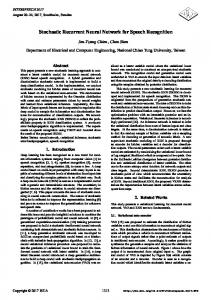
To recap, while most of the works in the GNN literature use a single graph with one type of diffusion [12, 14], we have proposed a (recurrent) multi-relational GNN architecture that: adapts to each graph with R; uses a simple but versatile recurrent tensor mapping (7); and includes several types of graph-based regularizers. 4. NUMERICAL TESTS Fig. 2: GRNN; L hidden (black) and one output (red) layers

3.2. Initial and final layers The operation of the first and last layers is very simple. Regarding ˇ (0) is defined using X as layer l = 1, the input Z ˇ(0) z ni = xn for all (n, i).

(8)

On the other hand, the output of our graph architecture is obtained by taking the output of the layer l = L and applying ˆ := g(Z ˇ (L) ; θg ), Y

(9)

ˆ is an N × K matrix, Yˆn,k repwhere g(·) is a nonlinear function, Y resents the probability that yn = k, and θg are trainable parameters. The function g(·) depends on the specific application, with the normalized exponential function (softmax) being a popular choice for classification problems. ˆ For notational convenience, the global mapping from X to Y dictated by our GRNN architecture –i.e., by the sequential application of (7)-(9)– is denoted as ˆ := Y

F(X; {θz(l) }, {θx(l) }, θg ),

(10)

and represented in the block diagram depicted in Fig. 2. 3.3. Training and graph-smooth regularizers The proposed architecture depends on the weights in (7) and (9). We estimate these weights by minimizing the discrepancy between the estimated labels and the given ones. Hence, we arrive at the following minimization objective ˆ Y) + µ1 Ltr (Y,

min (l)

(l)

{θz },{θx },θg

I X

ˆ > Si Y) ˆ Tr(Y

i=1

+µ2 ρ({θz(l) }, {θx(l) }) + λ

L X

kR(l) k1

l=1

ˆ = F(X; {θz(l) }, {θx(l) }, θg ). s.t. Y

(11)

In our classification setup, a sensitive choice for the fitting cost is PK ˆ Y) := − P ˆ to use Ltr (Y, n∈L k=1 Ynk ln Ynk the cross-entropy loss function over the labeled examples. Note also that three regularizers have been considered. The first (graph-based) regularizer promotes smooth label estimates over the graphs [5], and ρ(·) is an L2 norm over the GRNN parameters that is typically used to avoid overfitting [15]. Finally, the L1 norm in the third regularizer promotes learning sparse mixing coefficients and, hence, promotes activating only a subset of relations at each l. The backpropagation algorithm [18] is employed to minimize (11). The computational complexity of evaluating (7) scales linearly with the number of nonzero entries in S (edges), cf. (3).

We test the proposed GNN with L = 2, P (1) = 64, and P (2) = K. The regularization parameters {µ1 , µ2 , λ} are chosen based on the performance of the GRNN in the validation set for each experiment. For the training stage, an ADAM optimizer with learning rate 0.005 was employed [19], for 300 epochs2 with early stopping at 60 epochs3 . The multiple layers of the graph in this case are formed using κ-nearest neighbors graphs for different values of κ (i.e., different number of neighbors). This method computes the link between n and n0 based on the Euclidean distance of their features kxn − x0n k22 . The simulations were run using TensorFlow [20] and the code is available online4 . 4.1. Robustness of GRNN This section reports the performance of the proposed architecture under perturbations. Oftentimes, the available topology and feature vectors might be corrupted (e.g. due to privacy concerns or because adversarial social users manipulate the data to sway public opinion). In those cases, the observed S and X can be modeled as S =Str + OS

(12)

X =Xtr + OX .

(13)

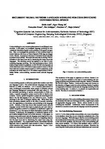
where Str and Xtr represent the true topology and features and OS and OX denote the corresponding additive perturbations. We draw OS and OX from a zero mean white Gaussian distribution with specified signal to noise ratio (SNR). The robustness of our method is tested in two datasets: i) A synthetic dataset of N = 1000 points that belong to K = 2 classes generated as xn ∈ RF ×1 ∼ N (µ, 0.4), n = 1, . . . , 1000 with F = 10 and µ = 0, 1 corresponding to the different classes. ii) The ionosphere dataset, which contains N = 351 data points with F = 34 features that belong to K = 2 classes [21]. We generate κ-nearest neighbors graphs by varying κ, and observe |L| = 200 and |L| = 50 nodes uniformly at random. With this simulation setup, we test the different GRNNs in SSL for increasing the SNR of OS (Figs. 3a, 3c) and OX (Figs. 3b, 3d). We deduce from the classification performance of our method in Fig. 3 that multiple graphs leads to learning more robust representations of the data, which testifies to the merits of proposed multi-relational architecture. 4.2. Classification of citations graphs We test our architecture with three citation network datasets [22]. The citation graph is denoted as S0 , its nodes correspond to different documents from the same scientific category, and Snn0 0 = 1 implies that paper n cites paper n0 . Each document n is associated with a feature vector xn that measures the frequency of a set of words, as well as with a label yn that indicates the document’s subcategory. 2 An

epoch is a cycle through all the training examples stops if the validation loss does not decrease for 60 epochs 4 https://sites.google.com/site/vasioannidispw/github 3 Training

κ =5

κ =10

κ =2

κ =5,10

1

Classification accuracy

Classification accuracy

κ =2

0.9 0.8 0.7 0.2

1

5

0.6 0.5 1

25

(b) Classification accuracy with noisy graphs. Classification accuracy

Classification accuracy

5 SNR of OS

(a) Classification accuracy with noisy features.

0.8

0.7

0.6 1

κ =5,10

0.7

SNR of OX

0.2

κ =10

0.8

0.2

25

κ =5

5

25

0.75 0.7 0.65 0.6 0.2

1

5

25

SNR of OS

SNR of OX (c) Classification accuracy with noisy features.

(d) Classification accuracy with noisy graphs.

Fig. 3: Classification accuracy on synthetic (a), (b) and ionosphere (c), (d). Dataset Cora Citeseer Pubmed

Nodes N 2,708 3,327 19,717

Classes K 7 6 3

Features F 1,433 3,703 500

|L| 140 120 30

Table 1: Citation datasets

“Cora” contains papers related to machine learning, “Citeseer” includes papers related to computer and information science, while “Pubmed” contains biomedical papers, see also Table 1. To facilitate comparison, we reproduce the same experimental setup than in [14], i.e., the same split of the data in train, validation, and test sets. We test two architectures: a) a GRNN using only the original citation graph S0 (and, hence, with I = 1); and b) a multirelational GRNN that uses an extra 1-nearest neighbor graph (so that I = 2). Table 2 reports the classification accuracy of various SSL methods. It is observed that: i) GNN approaches (ours, as well as [14]) outperform competing alternatives, ii) our GRNN schemes always outperform [14] (either with I = 1 or I = 2). This illustrate the potential benefits of the recurrent feed in (7) –not used in [14]– as well as the use of multi-relational graphs.

5µ

1

6µ

1

= 5 · 10−5 , µ2 = 5 · 10−5 , λ = 10−4 , dropout rate=0.9 = 2 · 10−6 , µ2 = 5 · 10−5 , λ = 10−4 , dropout rate=0.9

Method ManiReg [4] SemiEmb [9] LP [6] Planetoid [10] GCN [14] GRNN5 GRNN (multi-relational)6

Citeseer 60.1 59.6 45.3 64.7 70.3 70.8 70.9

Cora 59.5 59.0 68.0 75.7 81.5 82.8 81.7

Pubmed 70.7 71.7 63.0 77.2 79.0 79.5 79.2

Table 2: Classification accuracy for citation datasets

5. CONCLUSIONS This paper put forth a novel deep learning framework for SSL that utilized an autoregressive multi-relational graphs architecture to sequentially process the input data. Instead of committing a fortiori to a specific type of diffusion, our novel GRNN learns the diffusion pattern that best fits the data. The proposed architecture is able to handle scenarios where nodes engage in multiple relations, can be used to reveal the structure of the data, and is computationally affordable, since the number of operations scaled linearly with respect to the number of graph edges. Our approach achieves state-of-theart classification results on graphs when nodes are accompanied with feature vectors. Future research includes investigating robustness to adversarial topology perturbations, predicting time-varying labels, and designing of pooling operators.

6. REFERENCES [1] M. Kivel¨a, A. Arenas, M. Barthelemy, J. P. Gleeson, Y. Moreno, and M. A. Porter, “Multilayer networks,” Journal of Complex Networks, vol. 2, no. 3, pp. 203–271, 2014. [2] S. Wasserman and K. Faust, Social Network Analysis: Methods and Applications. Cambridge university press, 1994, vol. 8. [3] V. N. Ioannidis, P. A. Traganitis, Y. Shen, and G. B. Giannakis, “Kernel-based semi-supervised learning over multilayer graphs,” in Proc. IEEE Int. Workshop Sig. Process. Advances Wireless Commun., Kalamata, Greece, Jun. 2018. [4] M. Belkin, P. Niyogi, and V. Sindhwani, “Manifold regularization: A geometric framework for learning from labeled and unlabeled examples,” J. Mach. Learn. Res., vol. 7, pp. 2399– 2434, 2006. [5] V. N. Ioannidis, M. Ma, A. Nikolakopoulos, G. B. Giannakis, and D. Romero, “Kernel-based inference of functions on graphs,” in Adaptive Learning Methods for Nonlinear System Modeling, D. Comminiello and J. Principe, Eds. Elsevier, 2018. [6] X. Zhu, Z. Ghahramani, and J. D. Lafferty, “Semi-supervised learning using gaussian fields and harmonic functions,” in Proc. Int. Conf. Mach. Learn., Washington, USA, Jun. 2003, pp. 912–919. [7] D. I. Shuman, S. K. Narang, P. Frossard, A. Ortega, and P. Vandergheynst, “The emerging field of signal processing on graphs: Extending high-dimensional data analysis to networks and other irregular domains,” IEEE Sig. Process. Mag., vol. 30, no. 3, pp. 83–98, May 2013. [8] A. G. Marques, S. Segarra, G. Leus, and A. Ribeiro, “Sampling of graph signals with successive local aggregations,” IEEE Trans. Sig. Process., vol. 64, no. 7, pp. 1832–1843, Apr. 2016. [9] J. Weston, F. Ratle, H. Mobahi, and R. Collobert, “Deep learning via semi-supervised embedding,” in Neural Networks: Tricks of the Trade. Springer, 2012, pp. 639–655. [10] Z. Yang, W. W. Cohen, and R. Salakhutdinov, “Revisiting semi-supervised learning with graph embeddings,” in Proc. Int. Conf. Mach. Learn., New York, USA, Jun. 2016. [11] D. Berberidis, A. N. Nikolakopoulos, and G. B. Giannakis, “Adaptive diffusions for scalable learning over graphs,” arXiv preprint arXiv:1804.02081, 2018.

[12] M. M. Bronstein, J. Bruna, Y. LeCun, A. Szlam, and P. Vandergheynst, “Geometric deep learning: going beyond euclidean data,” IEEE Sig. Process. Mag., vol. 34, no. 4, pp. 18– 42, 2017. [13] F. Gama, A. G. Marques, G. Leus, and A. Ribeiro, “Convolutional neural networks architectures for signals supported on graphs,” arXiv preprint arXiv:1805.00165, 2018. [14] T. N. Kipf and M. Welling, “Semi-supervised classification with graph convolutional networks,” in Proc. Int. Conf. on Learn. Represantions, Toulon, France, Apr. 2017. [15] I. Goodfellow, Y. Bengio, A. Courville, and Y. Bengio, Deep Learning. MIT press Cambridge, 2016, vol. 1. [16] M. Defferrard, X. Bresson, and P. Vandergheynst, “Convolutional neural networks on graphs with fast localized spectral filtering,” in Proc. Advances Neural Inf. Process. Syst., Barcelona, Spain, Dec. 2016, pp. 3844–3852. [17] L. Ruiz, F. Gama, A. G. Marques, and A. Ribeiro, “Median activation functions for graph neural networks,” arXiv preprint arXiv:1810.12165, 2018. [18] D. E. Rumelhart, G. E. Hinton, and R. J. Williams, “Learning representations by back-propagating errors,” Nature, vol. 323, no. 6088, p. 533, 1986. [19] D. P. Kingma and J. L. Ba, “Adam: A method for stochastic optimization,” in Proc. Int. Conf. on Learn. Represantions, San Diego, CA, USA, May 2015. [20] M. Abadi, P. Barham, J. Chen, Z. Chen, A. Davis, J. Dean, M. Devin, S. Ghemawat, G. Irving, M. Isard et al., “Tensorflow: a system for large-scale machine learning.” in OSDI, vol. 16, Savannah, GA, USA, Nov. 2016, pp. 265–283. [21] D. Dheeru and E. Karra Taniskidou, “UCI machine learning repository,” 2017. [Online]. Available: http://archive.ics.uci. edu/ml [22] P. Sen, G. Namata, M. Bilgic, L. Getoor, B. Galligher, and T. Eliassi-Rad, “Collective classification in network data,” AI magazine, vol. 29, no. 3, p. 93, 2008.