A Recurrent Neural Network for Real-Time Computation of Semidefinite Programming Danchi Jiang, Jun Wang Department of Mechanical and Automation Engineering Chinese University of Hong Kong Shatin, N. T., Hong Kong
[email protected] [email protected] Abstract This paper proposes a novel recurrent neural network for the real-time computation of semidefinite programming. This network is developed to minimize the duality gap between the admissible points of the primal problem and the corresponding dual problem. By appropriately defining an auxiliary cost function, a modified gradient dynamical system can be obtained which ensures an exponential convergence of the duality gap. Then, two subsystems are developed to avoid the difficulties involving matrix inverse and determinant, so that the resulted dynamical system can be easily realized using an analog recurrent neural network. The architecture of the resulting neural network is also discussed. The operating characteristics and performance of the proposed approach are demonstrated by means of simulation results. The approach reported in this paper not only gives an promising way for real-time computation of semidefinite programming, but also offers several new insights for its numerical computation.
example, see [l, 3, 4, 91. There are many numerical algorithms reported to solve this problem and the literature is still quickly growing. See [4, 6, 8, 9, lo] and references cited therein. This paper will propose a recurrent neural network for real-time computation of it. Recurrent neural networks have been successfully applied to the real-time computation of many optimization problems. See [ll, 121 for some examples. One of the main ideas is to build an recurrent neural network such that the state of the neural network represents the decision vector of the optimization problem and the dynamics of the neural network reflects certain gradient descent property of the corresponding cost function. If the dynamics is realized using an analog circuit, the steady state can be reached quickly. In addition to this intuition, the effectiveness of the neural network developed in this paper is also established by theoretical results and demonstrated by simulation results.
1.1 Duality Gap The dual problem of the problem defined by (1) and (2) can be defined [8, 91 as:
1. Introduction Consider the semidefinite programming problem defined as: min s. t.
JP(x) = CTx, (1) := F0 + FIx1 + F2x2 + . . . + K&2 ,> o(2) F(z)
= E !JP c (x1,x2,* 4n) T Cn)T, Fi E S ( m ) C !J?“‘“, i(m) d e notes the set of all m x m symmetric matrices, and . i 2 = 0,1,2,. . . , n) are linearly independent. The F( constraint (2) means that F(x) is positive semidefinite. This problem can been widely applied to control design, combinatorial optimization, and other areas. For
where
x
l
(G,C2,**-,
O-7803-4859-1/98 $10.0001998 IEEE
1640
maximize
Jd(z)
subject to
tr(FiZ) = C&i = 1,2,. . . ,n;
(3) (4)
Z 2 0,
(5)
=
-tr(FoZ) Z E S(m).
To simplify the subsequent analysis, we need the following two assumptions: A-1 The cost function JP(x) is bounded below on the admissible set defined by {x E Rn : F(x) > O}. A-2 Both the primal problem defined by (1), (2) and the corresponding dual problem defined bY 6% (41, (51 are strictly feasible; i.e., there exist a vector x and a positive definite matrix Z such that F(x) > 0, tr(F;Z) = Ci, i = 1,2,. . . ,m. The first assumption is concerned with the consistency of the problem. In the case that this assumption
is not satisfied, the minimum of the cost is negative infinity. The second assumption is not a restriction on a semidefinite programming problem either. In fact, many techniques have been reported that can convert a semidefinite programming problem into a primal and dual strictly admissible one. For example, one can obtain a primal and dual strictly admissible semidefinite programming problem by the “big-M” method reported in [2]. It is worth to mention that by using the “big-M” method, one can also obtain an admissible solution to the original semidefinite problem if there exists one. It is shown in [8] that the following duality theorem holds: Theorem 1 (Duality Theorem) [8, page 1091 If the assumptions A-I and A-2 are satisfied, then, an admissible pair (x”, Z*) of the primal and dual problems defined respectively by (l), (i?), and (3), (4), (5) respectively is optimal if and only if tr(F(x)Z) = 0. tr(F(x)Z) is termed as a duality gap. The optimal solution can be computed by minimizing the duality gap since it is always non-negative at any admissible point. Indeed, this idea is used in many studies such as those reported in [8, lo]. One can justifies this approach by the following analysis. Note that the dual problem defined by (3), (4), and (5) can also be converted into the following form: Jd = DT x
min s. t .
G( x >
1.2 Central Trajectory Consider the minimization of the following cost function: Jp(x, z) = PGap - logdet(F(x)G(x)),
where ,0 > - 0. This cost function is strictly convex. As ,8 varies, the optimal solution of the unconstrained problem (12) defines a curve. This curve is called a central trajectory. Note that, as ,8 tends to +oo, the central trajectory converges to the optimal solution pair of the primal and dual problems defined by (l), (2) and (3), (4), (5), respectively. Based on the analysis of this problem, we obtain the following two properties concerning the central trajectory. Lemma 1 Consider the combined problem defined by (IO) and (11). (1). An admissible pair (x, x) is on the central trajectory if and only if F(x)G(x) = *I. m
where the following relations hold: Jd
=
- Jd - tr(FoGo),
D
=
(tr(FoG), tr(FoGz),
0 l
l
l
, tr(FoG>>T(s>
tr(FiGo) = Ci, i = 1,2,. . . ,n, tr(FiGj) = 0, i= 1,2 ,..., 72, j = 1,2 ,..., 1.
m”det(F(x)G(z)) 5 [Gaplm.
2 A Modified Gradient System 2.1
An Auxiliary Cost Function
Introduce an auxiliary cost function as follows:
a := tr(F(x)G(z)) = tr(FoGo) + CTx + DTz. GP Therefore, the primal and dual problems defined respectively by (1)) (2) and (3)) (4)) (5) can be solved simultaneously by solving the following problem:
subject to
Jc(x,x) = Gap
(10)
F(x) >- 0,
(11)
G(x) > 0
(14)
Proof. Omitted for brevity.
The duality gap, denoted as Gap in the rest of this paper, now becomes:
minimise
(13)
(2). For any admissible pair (x, z)
0
:= Go + Glxl + . . . + Glxl 2 0, (7)
(12)
This problem is larger than primal problem and its dual problem in terms of the dimension of the corresponding decision vector. However, it is known that its optimal cost value is zero, which provides an advantage for the development of appropriate optimization algorithms and the corresponding theoretical analysis.
1641
(15) f o r x E !J?, x E X1, s u c h t h a t F ( x ) > O,G(x) > 0 , v > 0 is an adjustable parameter. This auxiliary cost function has the following interesting properties: Lemma 2 Consider the auxiliary cost function defined bY (W (1). @(x,z) 2 0. (2). qw> L [GaPy”
(3).
If there is a sequence (xk, z”) such that a( xk,zk) + 0,
then this sequence converges to the optimal solution set of the semidefinite programming problem.
Proof. Clearly, by the positive definite property of F(x),G(x) and (14) in Lemma 1 one can obtain ( 1 ) and (2) . The last result is a direct conclusion of (2).
where !P is defined as
Based on these results in Lemma 2, we can search for an optimal solution by minimizing this auxiliary cost function. Note that any optimal solution to the semidefinite programming problem is a global one because the cost is convex. The gradient grad@(x) x) can be calculated by the techniques in [7] as
In fact, we consider the function XP is a switch. More specifically, when Gap = 0, we let the right hand side of (18) to be zero without computing grad@, which might be not well defined. Within any interval such that G a p > 0 the time derivative of @(t) can be calculated as
Y s> = 1 01
i&E
for s > 0, for s < - 0.
(19)
d@ li: = -yip+“. XT)ZT) a( ( 2 >
Hence the solution to the differential equation (20)) denoted as Q(t) for brevity, is solved as
w -- { Gap
(21)
Theorem 2 (Convergence Property) Suppose (x(0),x(O)) is an arbitrary initial point such that F(x(0)) > 0, G@(O)) > 0. (1). There exists a unique solution for the equation (18) in the time interval [0, +oo). Along the trajectory of (18) starting from (2) (2(0)‘~(0))7
A Neural Network Model
The minimal point of the auxiliary function (15) might be a local one since the function @(x, x) is not a convex function. Furthermore, in the case that the global optimal solution can be obtained, the corresponding algorithm converges only linearly or quadratically. In order to obtain the global optimal solution efficiently, we propose a modified gradient system to compute the semidefinite programming problem as folgrad@ ?’]]gradQi]12 “? for F(x) > 0, G(x) > 0,
if a = 0, if a > 0.
Therefore, by applying Lemma 2 we know that the solution of (18) exists for all time t E [0, +oo). Hence the following convergence property of the model (18) holds:
.- m+v P .- - .
2.2
W) e---Yt ay!}~
{[+(0)]--Ly +
and the cost function @(t) strictly decreases until an optimal solution to the combined problem given by (IO) and (II) is achieved; i.e., one of the inequalities in (22) violated and the duality gap becomes zero. (W If a = 0, along the trajectory there holds:
(17)
tr(F(x(t))G(x(t))) < [a(t)]5 = [a(O)]” e-St; w h e r e ]I I] is the F’robenius norm ( i.e., Ilgrad@]]” = [grad@lTgrad@ ), and a > 0, y > 0 are any parameters that can be chosen freely. Later in this paper one can see that a = 0 is preferred. In fact, the auxiliary cost function Q is an exponential function of the primal-dual potential reduction cost function addressed in [8, lo]. It is known [lo, Theorem 31 that for any strictly feasible point (x, x), grad@ # 0. Therefore, the definition of (17) is justified. We extend the definition of (17) to more general cases as follows: l
i. e., the duality gap converges to zero exponentially. If a > 0, then tr(F(x(t))G(x(t))) 5 [mm@(t)]* = rt-‘, where
&=E 3/ = [my]? v’
Proof. (1) Only two cases can happen: Case 1, Gap > 0 along the trajectory of (18). Then, (x, x> remains strictly feasible, the solution to (18) exists in the interval [0, +oo) and @ satisfies (20) all the time.
grad+
:= -r’(GaP) llg r a#,I12 ‘l+? 1642
Case 2, G a p > 0 will be violated at some time. Then, there is a time interval [0, b) such that Gap > 0 for t E [0, b) a n d tr(F(x(b)x(b)) = 0 . T h e n , x(t) = x(b)7 dt> = x(b) for t > b. (1) is established. (2) and (3) can be clearly seen from the argument for (1) and the formula of @ given by (21).
Let the matrix [Gap]m+“[F(x)G(x)]-l be denoted as W(t). Then, its derivative with respect to time is calculated as: . m+v T* T* w(t) = tr(F(x(t)G(x(t))) (’ x ’ D z)w(t) - Gap-(m+“) 2 W(t)FiG(z(t))W(t)&
3 Realization of the Neural Network
i=l
Model
-Gap-(“+“) x W(t)F(x(t))GjW(t)ij,
Note that the modified gradient flow (18) is, in fact, not ready yet for realization as an analog neural network because of the difficulties in the computation of the determinant and inverse of F(x) and G(x) contained in the gradient and a. In this section, we will discuss how to cope with those difficulties and present a neural network for the computation of semidefinite programming.
where ?, i are given by (18). The time-varying matrix W(t) can also be determined by using the dynamical system (24) and the initial condition: W(O)
(25)
= -+P(Gap)Gapm+“‘@) F, ( 2 6 ) IlW II2 = -+P(Gap(Qi(t))‘+“, @(O) = @(xo,xg), (27)
. w>
Instead of computing the inverse (F(x)G(z))-1 or (F(x)Y > wwl, we construct a recurrent neural network to compute [Gap]m+v[F(x)G(z)]-l. The reason lies in the following result:
where V(t) := (m + u)Gapm+u-l
Lemma 3 Along the trajectory of (18) starting from any strictly admissible pair (x0, ZO), t+b-
= [tr(F(xo)G(~o>)]m+“(F(zo>G(~o)>-l.
Furthermore, we can also compute i and 2 by the following formula which is equivalent to (18):
3.1 Computation of the Inverse of an TimeVarying Matrix
lim [Gap]m’VIF(x)G(x)]-l = 0,
(24)
j=l
-
(28)
(23)
where b is +oo or a positive real number corresponding to Case I or Case 2, respectively, in the proof of (1) of Theorem 2. Proof Let the eigenvalues of [F(x(t))G(z(t))] be denoted as Ar (t) 5 X2 (t) < . . . < Am. Since
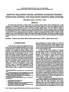
3.2 Neural Network Architecture Based on the previous discussion, we can build a neural network associated with the dynamical s y s t e m (24), (26), a n d ( 2 7 ) . F o r t h i s r e c u r r e n t neural network, the computation of the determinant det(F(x(t))G(z(t))) and the matrix inverses (F(wl > wwl are avoided by computing @ and W using their dynamical systems. See Figure 1 for a simplified block diagram. The corresponding electronic circuits of those sub-networks can be easily obtained because the computation is only a combination of addition, subtraction and multiplication of x, x and a switch circuit realizing the binary (hard-limiting) function. It is worthy noting that the initial condition for x, x and W, @ are not independent. More specifically,
F(x)G(x) = [F(x)]*([F(~)]+G(~)[F(~)~]+)[F(~)]-t, all eigenvalues of F (x)G(x) are simple and positive. Then, from (14) we know that [Gap]m+v $ = [Gap]“+” detFt)2(z)) = mm@(x, z) fi Xi i=2
< mm@(x,z)[Gaplm-’ ---+ 0, ast--+b-.
qjo -
Since [Gap]“+” & is the largest eigenvalue of the matrix [Gap]m+v [F(x)G(z)]-l, the proof is complete. m
1643
w o
=
~w(xoFhmm+u ; det(F(xo)G(~o))m”
( tr ( ~ ( x o >G( ~ o >>>““+“( G( z o >>l
( F ( x o ) ) l
l
(29)
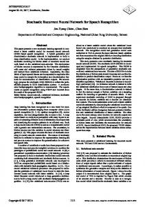
Figure 2. Duality gap converges to zero exponentially along the trajectory of the dynamical system defined by (24), (26) and (27).
Figure 1. Simplified block diagram for the composite model (24), (26) and (27). In this diagram, I, II, III, IV stand for four subnetworks that compute 6, i, I/t-, and 2, respect ivel y.
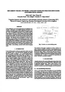
Figure 3. Duality converges gap to zero exponentially along the trajectory of the dynamical system defined by (18) where matrix inverses are computed by using a build-in function of Matlab.
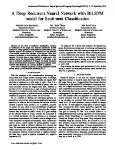
is much slower to obtain a solution with respect to the same precision required in the computation described above, as shown in Figures 3. This is due to the error generated in the computation of inverses of nearsingular matrices. In the analysis of our approach, we assume that the initial condition of W(t) and a(t) are precisely the results of formulas (29). In practice, we can only get an approximate value of it. To demonstrate the effectiveness of our approach, we have done a simulation with one percent error in the initial condition. The simulation results show in the Figures 4 that the computation error of the initial condition of W and @ can be neglected. It would be an interesting topic for furthermore investigation concerning the theoretical aspects of this phenomenon.
4 Simulation Results In this section, simulation results are given to demonstrate the efficiency of the proposed approach. First, we generate a problem randomly. For the illustration purpose, we choose the dimension of the positive definite matrices as 3 and the number of the primal decision variables as 4. Then we randomly generate an admissible primal semidefinite problem and use the “big-M” method to obtain a dual admissible problem. In order to demonstrate the convergence property of the proposed neural network, we solve the trajectory of the modified gradient system (18) numerically. The simulation result is plotted in Figures 2. In Figure 2, one can see that the duality gap rises first then converges to zero exponentially. The increasing is the effect of the determinant factor in the auxiliary cost function (15). Simulation also shows that the primal and dual variables converge to their steady states quickly. In the auxiliary cost function @, v is a weighting factor that adjustable. It is possible that we can keep the duality gap to be positive all the time by adjusting this parameter. Our Simulation experiments suggest that this can happen. As mentioned before, W ( t ) is used instead of Pwwrl t o avoid the computation of the inverse of a matrix that is close to singular. To demonstrate the effect of this idea, we have also computed the trajectory of the modified gradient system (18) directly. It
5 Concluding Remarks We have proposed a recurrent neural network approach to semidefinite programming. We first constructed an auxiliary cost function reflecting both the minimization of the duality gap and the satisfaction of the linear matrix inequality constraint. Then, we proposed a modified gradient dynamical system based on this auxiliary cost function. Following any trajectory of this system starting from any strictly primal-dual feasible point, the duality gap converges to zero exponentially. Then, two subsystems are introduced so that the resulted dynamical system can be easily re-
1644
of the dynamical system of x(t), x(t), W(t), a(t) in this paper clearly suggests an iterative procedure. It would be a very interesting issue to analyze the property of the corresponding algorithm.
Purturbation on the duality gap along the trajectory 18-
References [l] F. Alizadeh, 1995, Inter point methods in semidefinite programming with applications to combinatorial optimization, SIAM Journal on Optimization, vol. 5, pp. 13-51.
6-
[Z] M. S. Bazaraa, H. D. Sherall, and C. M.Shetty, 1993, Nonlinear Programming. Theory and Algorithms. second edition. Wiley, New York.
420 0
I 5
I 10
I 15
20
[3] S. Boyd, L. El Ghaoui, E. Feron, and V. Balakrishnan, 1994, Linear matrix inequalities in System and Control Theory. vol. 15 of Studies in Applied Mathematics, SIAM, Philadelphia.
I 25
Figure 4. Duality gap converges to zero exponentially along the trajectory of the dynamical system defined by (24), (26) and (27) where initial condition of W and