A representation for comparing simulations and ... - CiteSeerX

Artificial Intelligence for Engineering Design, Analysis and Manufacturing ~2001!, 15, 189–201. Printed in the USA. Copyright © 2001 Cambridge University Press 0890-0604001 $12.50

A representation for comparing simulations and computing the purpose of geometric features

THOMAS F. STAHOVICH and LEVENT BURAK KARA Mechanical Engineering Department, Carnegie Mellon University, Pittsburgh, PA 15213, USA (Received January 26, 2000; Accepted May 3, 2000!

Abstract We present a new representation that allows a rigid-body dynamic simulation to be described as a set of “causalprocesses.” A causal-process is an interval of time during which both the behavior and the causes of the behavior remain qualitatively uniform. The representation consists of acyclic, directed graphs that are isomorphic to the flow of causality through the kinematic chain. Forces are the carriers of causality in this domain; thus they are central to the representation. We use this representation to compute the purposes of the geometric features on the parts of a device. To compute the purpose of a particular feature, we simulate the behavior of the device with and without the feature present. We then re-represent the two simulations as causal-processes and identify any causal-processes that exist in one simulation but not the other. Such processes are indicative of the feature’s purpose. Because they are already causal descriptions of behavior, they can be directly translated into natural language descriptions of the feature’s purpose. We have implemented our approach in a computer program called ExplainIT II. Keywords: Causal Reasoning; Causal Representation; Design Rationale Construction; Computing Purpose; Simulation

alternatives considered, and a description of the intended purpose of each part of the design. Our work is concerned with the latter type of information, which is necessary for modifying a design without introducing unintended side effects. This kind of information is essential for resolving conflicts in distributed and collaborative design, for modifying a design to make it more easily manufacturable, for redesigning a product to add new ~marketing! features, and for adapting an existing design to a new application. Towards our goal, we are building a computer program called ExplainIT II that can compute the purposes of the geometric features on the parts of a device. We have focused on features because our informal analysis has revealed that that is what people typically do. It is common to find documentation of the form “the notch on part X is intended to . . .” As further justification, work by Knuffer and Ullman ~1990! indicates that questions about the construction, purpose, and operation of features are among the questions most frequently asked by professional engineers during a redesign exercise. In the design speaking-aloud protocol studies they conducted, over 25% of the questions concerned features. The importance of features in understanding the operation of a device is not surprising when

1. INTRODUCTION This paper describes a representation of mechanical behavior that allows a computer program to construct explanations for the purposes of the geometric features on the parts of a device. This work is motivated by the desire to decrease the cost of documenting a design. Good documentation is essential for performing a variety of common tasks during the product life cycle; however, creating good documentation places a significant burden on the designer. Furthermore, it is usually not the designer, but rather others downstream in the product life cycle, who benefit from this effort. Our goal is to create methodologies for automatically computing particular types of documentation. There are a variety of different kinds of information commonly included in design documentation. For example, it can contain a history of the decision-making process, a list of the

Reprint requests to: Thomas Stahovich, Mechanical Engineering Department, Carnegie Mellon University, Pittsburgh, PA 15213, USA. E-mail: [email protected]

189

190 one considers that if the designer bothered to create a feature, it most likely has some intended purpose. ExplainIT II builds upon our previous work with our earlier ExplainIT system ~Raghavan & Stahovich, 1998; Stahovich & Raghavan, 1999!. The two systems rely on the same basic principle. They compute the purpose of a feature by comparing a simulation of the nominal device ~“nominal simulation”! to a simulation of the device with the feature removed ~“modified simulation”!. The difference between the two computer systems is how they implement this principle: ExplainIT compares behavior directly while ExplainIT II compares a causal description of the behavior. ExplainIT uses heuristics for identifying specific pieces of the nominal simulation that must be compared to specific pieces of the modified simulation. These heuristics, however, were designed to handle only “state-change” devices— devices whose purpose is for the parts to start in one position and end up in another.1 ExplainIT II, on the other hand, is intended to handle a much broader range of devices, including those that operate cyclically. For these kinds of devices, the program must compare the two simulations behavior by behavior. The main difficulty is determining when two pieces of behavior are the same. For example, a particular behavior may occur multiple times during a simulation, and it is difficult to determine which instances from one simulation match which instances from the other. Our solution to this problem relies on the simple yet powerful insight, that for two behaviors to be the same, they must have the same cause. To implement this insight, we had to develop a new representation for describing causality in mechanical systems. We call our representation “causal-processes.” A causal-process is a description of behavior combined with a description of the causes of the behavior. The purpose of the feature can be determined by identifying all of the causal-processes that occur in the nominal simulation but not the modified one, and vice versa. These processes can then be directly translated into text, providing human-readable explanations of purpose. Consider, for example, the shutter mechanism of the single-use camera in Figure 1. When the feature on the end of the hook is removed ~Figure 2! and a new simulation is performed, we find that there are two causal processes that are unique to the nominal simulation. One is the lever causing the hook to be depressed and released while the lever is being cocked. The other is the hook causing the lever to remain at rest prior to when the shutter release button is pressed. Thus, the feature on the hook has two purposes: One is to enable the lever to displace the hook during cocking and the other is to restrain the lever after it is cocked.2 The bulk of this paper focuses on our new causal-process representation, beginning in Section 3. This is proceeded, however, by further background on the approach used by 1 A mechanical pencil is a common example of a state-change device: When the eraser end of the pencil is pressed and released, the lead moves forward a small distance, that is, the lead changes state. 2 The details of this example are provided in Section 4.

T.F. Stahovich and L.B. Kara

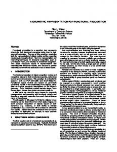
Fig. 1. The shutter mechanism of a single-use, 35 mm camera. To cock the camera, the user turns a wheel and winds the film onto a spool ~not shown!. As the film moves, it turns a gear, thus applying torque T to the cam. The cam cocks the lever which is then held in place by the hook. To snap a picture, the user presses the shutter release button ~not shown!, applying force F to the hook, releasing the lever, and snapping the shutter blade. In the position shown, one arm of the lever is just about to depress the hook, while another arm is just about to slip past the shutter blade. The shutter blade has two degrees of freedom. It can translate down during cocking to allow the arm of the lever to pass by without exposing the film. When the picture is snapped, the arm of the lever engages the blade so as to rotate it and expose the film.

the original ExplainIT system. Additionally, Section 5 places our current work in the context of related work. We have implemented the portion of ExplainIT II that uses our new representation to identify those differences between the nominal and modified simulations that are indicative of a feature’s purpose. Section 4 briefly describes how this computation is performed. It also describes how the differences can be translated into natural language descriptions of purpose, although the code for doing this latter task is only partially implemented. 2. BACKGROUND: THE PREVIOUS ExplainIT SYSTEM Simulations describe what happens but not why. Thus, a simulation does not directly indicate which of a device’s many behaviors are caused by a given feature on a given part. To identify those behaviors, ExplainIT compares a simulation of the nominal device to a simulation with the

Fig. 2. ~A! The hook. ~B! The hook with the feature removed. The hook is modeled as a translating body connected to a spring.

A representation for computing purpose feature removed. The differences between them are indicative of the behaviors the feature ultimately causes. One of the challenges in implementing this approach is determining which of the differences are significant. Direct numerical comparison of the state variables is not useful because there are likely to be differences in force magnitudes, velocities, accelerations, and so forth at every instant of time. Many of these differences are insignificant, such as those resulting from the small change in mass that occurs when the feature is removed. To have a reliable definition for which differences are important, ExplainIT is restricted to state-change devices ~devices whose purpose is for the parts to start in one position and end up in another!. For these types of devices, differences between the final states of the simulations are the significant ones. Thus, when comparing the nominal and modified simulations, ExplainIT starts by identifying the bodies whose final state is qualitatively different between the two simulations. The program characterizes the final state of a body in terms of the sign of its net displacement. If there is a positive net displacement in one simulation and no net displacement in the other, for example, the body’s final state is considered different. For each such body, the program must find the first point at which the behavior begins to differ between the simulations. This is the point when the feature must perform its intended purpose in order to make the body end up in the correct final state. The program segments the motion of the body into intervals of uniform motion: periods during which the velocity remains strictly positive, strictly negative, or zero. The program then identifies the first pair of corresponding segments whose velocities have different signs. For example, if the first four segments of the two simulations match, but the fifth segments do not ~e.g., the velocity in one is positive while that in the other is negative!, then the start of the fifth segment is where the feature performs its purpose. ExplainIT assumes that the difference in velocity is due to new forces that appear, or old forces that disappear, when the feature is removed. The next step in the analysis is to compute a causal explanation for these forces. If a new force appears in the modified simulation, the program uses the laws of mechanics to determine how the surfaces created by removing the feature cause the force to exist. Conversely, if a force appears only in the nominal simulation ~i.e., the force disappears in the modified simulation!, the program uses the same laws to determine how the surfaces of the feature cause the force to exist. To complete the analysis, ExplainIT directly translates these causal explanations into human understandable descriptions of the feature’s purposes. It does this by using pre-written text templates to translate the components of the causal explanation ~the causal-links! into English text. ExplainIT is intended to be used by the designer when a design is nearly completed. The system would attempt to document the purposes of all of the features on all of the parts. ~The features would be provided by a separate feature identification and removal tool.! If ExplainIT is un-

191 able to identify the purpose of a particular feature ~there are no differences between the simulations when the feature is removed!, the program would have to prompt the designer for one. There are three possible outcomes in this case. The first is that there really is no purpose, in which case the program has identified an opportunity to simplify the design by removing the feature. The second is that there is a purpose, but it is a subtle one. For example, the feature may have nothing to do with the operation of the device, but might instead be an artifact of a specialized manufacturing process. In this case, the program would be prompting the designer for an explanation that perhaps only he or she would know. This kind of explanation is particularly valuable and the program would have performed a useful service by drawing the designer’s attention to it. ExplainIT’s goal is to document all of the obvious purposes and to focus the designer’s attention on the subtle parts of the design, which makes for efficient use of the designer’s time. The third case is that the purpose is related to physics in other domains such as heat transfer or fluid mechanics. When this occurs, the designer will have to manually document the purpose. 3. REPRESENTATION The primary challenge in implementing our remove and simulate technique is accurately identifying the differences between the nominal and modified simulations. Consider, again, the purpose of the hook in the shutter mechanism of the single-use camera in Figure 1. Recall that when the feature on the end of the hook is removed ~Fig. 2!, the camera’s operation is quite different from its ordinary operation: the hook is not deflected while the lever is being cocked, and the lever is not restrained by the hook prior to when the shutter release button is pressed. ExplainIT’s heuristics would not be able to determine the purpose of the feature in this case because the shutter mechanism operates cyclically. Even when the feature on the hook is removed, the camera still ends up in the correct final state. ~Of course, without the feature, the shutter blade would snap early and a different picture would be taken.! In this problem, the final states give no clues about the purpose of the feature on the hook and thus we must somehow compare the two simulations behavior by behavior. Unfortunately, a direct comparison of behavior is fraught with ambiguity. The difficulty is accurately determining when two behaviors are the same. Notice that when the nominal device is operated through a complete cycle, the hook moves down two separate times ~once while the lever is being cocked and once when the shutter release button is pressed!. But when the feature on the hook is removed and the device is again operated, the hook moves down only once. The challenge is determining if the down stroke in the modified simulation is the same as either of those in the nominal simulation. Chronology provides little help in this matter. The strokes occur at very different times in the two simulations. In the nominal simulation, both strokes occur be-

192 fore the shutter blade is snapped, but in the modified simulation the stroke occurs after. If we considered elapsed time, rather than the sequencing of events, we would correctly identify which strokes match. However, using elapsed time would produce a different, and perhaps bigger, set of problems. For example, the shutter blade snaps at a much earlier elapsed time in the modified simulation than it does in the nominal one. Thus, based on elapsed time, we would incorrectly conclude that the two behaviors are different. In some cases, chronological order gives the right answer, and in others the elapsed time does. However, there is no way to know a priori which to use in any particular circumstance. Because temporal analysis is inadequate to disambiguate behaviors, we set out to identify some other means to accomplish this task. Our solution relies on the simple yet powerful insight that for two behaviors to be the same, they must have the same cause. For example, the second down stroke of the hook in the nominal simulation is the same as the down stroke in the modified simulation because both strokes have the same cause, the externally applied force F. For our program to use this insight, we had to develop a new “causal-process” representation to allow the program to describe a mechanical simulation as a sequence of processes with associated causes. The sections that follow provide a complete discussion of this representation, including what a causal-process is, how causality is determined, and how we implement these concepts in a computer program.

3.1. Causal-processes A causal-process is an interval of time during which both the behavior and the causes of the behavior remain qualitatively uniform. Because we are examining rigid-body dynamic simulations, our causal-process representation is designed to describe rigid-body dynamic behavior. Furthermore, we distinguish between two kinds of causal-processes: those that keep an object in equilibrium ~static processes! and those that keep an object in motion ~dynamic processes!. However, in both cases, we use the same principles to reason about causality: According to Newton’s laws, force causes ~or prevents! motion. We represent a dynamic process as an acyclic, directed graph that is isomorphic to the flow of causality through the kinematic chain. The nodes in the graph represent bodies, springs, and external forces. The arcs describe the causal relationships between the nodes. There are two types of arcs: An arc can represent one object causing another to move, or an arc can represent an object causing a spring to store potential energy.3 3 Springs are the only sources of potential energy we have considered. However, in principle, gravitational potential energy could be handled in the same fashion as springs. In fact, it is easier to track the sources of gravitational potential energy than it is to track those of elastic potential energy. To do the later reliably, we have to restrict springs to having one end fixed.

T.F. Stahovich and L.B. Kara

Fig. 3. A simple mechanical system: External force F acts to the right. Blocks A and B slide horizontally on a surface with friction.

The nature of causality in this domain places constraints on the structure of the graphs describing dynamic processes. External forces are always root causes of motion because nothing within the system causes an external force. Thus external force nodes have only outgoing arcs. For reasons described below, we assume that springs always have one end fixed ~this simplifies the task of tracking the origins of the spring’s potential energy!. Because of this assumption, spring nodes will have either all outgoing arcs or all incoming arcs, but not both. If the arcs are outgoing, the spring is causing other objects to move. If the arcs are incoming, other objects are causing the spring to store potential energy. Nodes representing bodies can have both outgoing and incoming arcs: The incoming arcs are from the objects causing the body to move, while the outgoing arcs point to the objects the body is causing to move ~or store potential energy!. To implement our representation we had to develop rules for tracking the flow of causality through a device. In our pursuit of these rules, we were able to make use of some results obtained by Sacks and Joskowicz ~1993!: They examined a large catalog of mechanisms and found that a significant fraction of them can be accurately modeled with an assumption of negligible inertia. We take advantage of this fact to greatly simplify the task of determining the causes of a body’s motion. If inertia is negligible, a body’s motion is caused by those forces having a component in the direction of motion.4 To illustrate this rule, consider the system shown in Figure 3 consisting of two blocks ~A and B!, an external force ~F!, and a spring ~S!. At the instant shown, A and B are touching and moving to the right while the spring is being compressed. We begin by examining body A. It experiences three forces: Force F pushes A to the right while the contact force from B and the friction force from the horizontal surface push A to the left. Only force F is in the direction of motion, thus it is the cause of motion. Similarly, because the force A applies to B is the only force in the direction of B’s motion, it is the cause of B’s motion. Finally, because B is doing work on the spring, B is the cause of the increase in the spring’s potential energy. Combining these results, we get the graph shown in Figure 4. It is apparent from the graph that our rule for causality does match our common sense notion of cause and effect: The 4 If inertia is appreciable, it is still possible to determine causality; however, doing so requires several special case rules. See Section 6.

A representation for computing purpose

193 3.2. History

Fig. 4. The dynamic process describing the behavior in Figure 3. Arcs labeled “push” indicate one object pushing another. Arcs labeled “ PE” indicate an object causing a spring to store potential energy. ~This is a simplified graphical depiction. The actual representation contains additional information including the fact that this is a dynamic rather than static process. See Section 3.3.!

graph indicates that F pushes A, which then pushes B, which then causes the spring to store potential energy. It is important to note that our causal graphs are not free-body diagrams. For example, the force B applies to A is not shown in Figure 4, as it would be in a free-body diagram, because it is not causing A to move. Similarly, if the situation were such that the spring force was strong enough to overcome force F, the resulting causal graph would not contain F. Instead, it would have an arc from S to B and one from B to A indicating that the spring was causing the blocks to move to the left. Every time a collision occurs, one dynamic process ends and a new process begins. The new process may be either dynamic or static. Imagine, for example, that blocks A and B in Figure 3 are initially separated. When force F is applied, there will be a dynamic process with F pushing A. When A collides with B, this initial process will cease and the one in Figure 4 will occur. Because the first graph is a subgraph of the second, and the two graphs have the same root, it is straightforward to determine that this second process is a continuation of the first. The rules of causality for static processes are much simpler than for dynamic processes. When a body is in static equilibrium, all of the forces applied to it are the cause of it being stationary. Thus, the graph describing a static process is a star with all of the arcs pointing toward the center. Consider again the two blocks in Figure 3. If they are at rest and force F exactly balances the spring, there will be two static processes as shown in Figure 5. In the first process, external force F and the force from B keep A in equilibrium. In the second process, the spring force and the force from A keep B in equilibrium.

Fig. 5. The static process representation describing the behavior in Figure 3 when force F and the spring exactly balance and the blocks are at rest. ~This is a simplified graphical depiction. The actual representation contains additional information including the fact that this is a static rather than dynamic process. See Section 3.3.!

Sometimes causes and effects may be separated in time. There are two situations in which this occurs in our domain. The first is when a dynamic process ~or processes! stores potential energy in a spring, and sometime later the spring releases the potential energy, thus initiating a new process. Consider once again the system in Figure 3. Imagine that after force F has pushed the blocks some distance to the right, the force is turned off and a latch ~not shown! engages and restrains the blocks. If the latch is later disengaged, the spring will push the blocks back to the left. The spring is able to do this precisely because the process in Figure 4 stored potential energy in the spring. ~Recall that in the initial state the spring was relaxed, thus all of the potential energy originated at F.! Thus, even though the two processes—force F pushing everything to the right and the spring pushing everything to the left—are separated in time, the first process is the cause of the second. We represent this kind of causal link by recording the history of the potential energy of each spring. The history is described as the list of causal-processes that supplied potential energy to the spring. As the spring relaxes and the potential energy is released, processes are removed from the history in a last-in-first-out fashion. For example, once the spring pushes the blocks back to the left in Figure 3, the spring will no longer have any potential energy from the dynamic process in Figure 4. Thus, this process will be removed from the history list. The reason we can use this last-in-first-out approach to tracking potential energy is our assumption that springs always have one end fixed. Without this assumption it would be possible for a process at one end of the spring to be supplying potential energy at the same time another process at the other end removes it. In that case, a simple list of processes would be inadequate to describe the history of the potential energy. Sometimes springs have potential energy when the device is in its initial state ~i.e., at the beginning of the simulation!. We represent this by use of a fictitious process we call the initial condition ~IC! process. For example, if the spring in Figure 3 was compressed in the initial state, the history list would initially contain the IC process. After the force pushed everything to the right, the list would contain two processes: Some of the potential energy would be attributed to the initial conditions, and the rest would be due to the process in Figure 4. The other situation in which cause and effect are separated in time is when a process ~or processes! puts a body in a particular location, thereby enabling a future process to occur. This situation occurs in the single-use camera ~Fig. 1!, for example. As the cam cocks the lever, the lever pushes the hook down. When the lever disengages the hook, the hook returns to its relaxed position, that is, a position that can block the lever’s path. Later, when the cam disengages the lever, the lever begins to move back toward the shutter blade, but because the hook is in the way, the lever gets

194

T.F. Stahovich and L.B. Kara

trapped. In this case, it is clear that one cause of the lever being trapped is the process that previously placed the hook in the lever’s path. We represent this kind of time-delayed causal link by recording the history of how each body arrived at its present location. We do this by maintaining a list of the processes that caused the body to be where it is. This list contains all of the dynamic processes that the body has experienced. If the last process the body experiences is a static process, that process is also included in the list because it is one of the reasons the body is where it currently is. Static processes that occurred earlier are not included in the list because they did not cause the body to be where it is. In fact, those processes temporarily prevented the body from getting to its present location. 3.3. Syntax We have implemented our representation in a LISP program and consequently our representation has the LISPlike syntax shown in Table 1. This section describes our implementation in the order in which its parts are listed in the table. We represent a simulation as a list of states in chronological order. A state is an interval of time during which the set of active causal-processes is constant. Each state contains a list of processes and a list of the events that occurred when that state began. The two different types of causal-processes are represented differently. The representation of a static process

Table 1. The LISP-like syntax of our causal-process representation simulation state process root link event

body force

why-there

source-of-PE

(^sim-name& [state]) (^state-name& [event] [process]) (STATIC ^body& [force] [why there]) (DYNAMIC [root] [link]) (^force& PUSHES ^body&) (^body-name& PUSHED-BY [body] PUSHES [body] ) (^spring-name& GIVEN-PE-BY [body]) (IC) (COLLISION ^body 1& ^body 2& ^why-there 1& ^why-there 2&) (DISENGAGEMENT ^body 1& ^body 2&) (INPUT-APPLIED ^name&) (INPUT-REMOVED ^name&) ^body-name& (EXTERNAL-FORCE ^name&) (SPRING-FORCE ^name& ^source-of-PE&) (CONTACT-FORCE ^name& ^why-there&) [process] (IC) (RIC [process]) [process] (IC)

Notation: ^type& is one object of type “type”. @type# 5 a list containing one or more objects of type “type.” All names ~e.g., ^body-name& and ^name&! are text strings. Items in all capital letters ~e.g., STATIC and IC! are special tokens.

contains a reference to the body that is in static equilibrium and a list of the forces that keep that body in equilibrium. The why-there part of the representation is the history list describing how the body arrived at its position. ~See Section 3.2 for a discussion of history lists.! The graphs representing dynamic processes are described implicitly with a list of root nodes and a list of links. The root nodes represent the root causes of motion, such as force F in Figure 3. A graph can have multiple root nodes because there can be multiple spring forces and external forces pushing a given body ~either directly or through a kinematic chain!. Root nodes contain a reference to a force ~either a spring force or an external force! and a reference to the body to which that force is applied. There are two types of links: One type describes a body pushing other bodies, the other type describes a body causing a spring to store potential energy. An event is an instantaneous occurrence that marks the end of one or more processes and the beginning of new processes. In our domain there are four kinds of events: Two bodies can collide, two bodies can separate, an external force can be applied, and an external force can be removed. We also define a fictitious initial condition event indicating that a process began in the initial conditions of the simulation. Collision events include history lists ~whythere! describing how the two colliding bodies arrived in positions that allowed them to collide. In our domain, there are three types of forces: external forces, spring forces, and contact forces. ~Contact forces appear only as part of a static process. For dynamic processes, contacts between bodies are represented by links.! Each external force has a unique name, which helps in determining when processes from different simulations are really the same. Spring forces contain a history list describing the origins of the potential energy. Contact forces contain a history list describing how the body arrived in a position such that it can apply a contact force. ~Note that “external forces” and “spring forces” can be either forces or torques.! A why-there history list describes how a body arrived in its current position. If a body is where it is because it has not left its initial position, the history list contains just one item: ~IC!. If the body has left the initial conditions and has not returned, the history list will contain a list of processes described in the usual way.5 If the body returns to its initial position, the list of processes describing the history is preceded by a special token, RIC. This provides a convenient way to reason about cyclic behavior. The source-of-PE history list is similar to the why-there history list, except that there is no need for the special RIC history list. Recall that as potential energy is lost, processes are removed from the history list.

5 When examining why a body is where it is, we need to consider only those nodes in a dynamic-process graph that can reach the body through the directed arcs. The “PUSHED-BY” list included in each link is used to identify the relevant portions of the graph.

A representation for computing purpose

195

4. USING THE REPRESENTATION

though both root nodes represent the same spring force, the history lists describing the sources of the spring’s potential energy are different in the two cases. In the first case the potential energy originates with torque T and in the other it originates with force F. Performing the complete comparison process on the camera example reveals a total of four unique processes. The first is shown in Figure 6. Part ~a! of the figure is a graphical depiction of the relevant dynamic process from the nominal simulation. This process has two branches as shown in part ~b! of the figure. In the first branch, the torque turns the cam, which pushes the lever, and causes the leverspring to store potential energy. In the second branch, the torque turns the cam, which pushes the lever, which pushes the hook, and causes the hook-spring to store potential energy.6 The relevant process from the modified simulation has a single branch, which is identical to the first branch from the nominal simulation. There is no match for the second branch. Thus, the second branch, when combined with the three other unique processes, indicates something about the purpose of the feature on the hook. Part ~c! of the figure shows this branch in the syntax of Section 3.3, and part ~d! shows it formatted for ease of reading. Figure 7 shows two other process that are unique to the nominal simulation.7 The first is the hook moving toward its relaxed position after the lever has released it. The second is the hook remaining in static equilibrium after reaching this relaxed position. The fourth difference between the two simulations is shown in Figure 8. This static process describes the lever stopped against the hook after the lever has been cocked and released by the cam, and after the hook has been depressed and released by the lever. Once all of the processes unique to one or the other of the two simulations have been identified, the final task is to translate them into a natural language explanation of purpose. We have implemented the code that identifies the unique processes. In fact, Figures 6d, 7, and 8 are output from our program ~with some manual formatting!. However, we have not yet completely implemented our code for generating the explanations from the unique processes. The goal of the work presented here was to verify that our representation is adequate for identifying those differences between the simulations that are indicative of the feature’s purpose. Having accomplished this goal, we are currently in the process of implementing code for generating the explanations of purpose. The remainder of this section provides a brief overview of the approach we are implementing. When generating explanations of the feature’s purpose, we refer to those processes that are unique to the nominal

Once the two simulations have been re-represented as causalprocesses, comparing the nominal and modified simulations is a straightforward process. The task is to identify all of the causal-processes that are unique to one or the other of the two simulations. These are the processes that are indicative of the feature’s purpose. To perform this task, it is necessary to check each process from one simulation to see if it has a match in the other. To compare two static processes for a possible match, we simply check if the two pieces of the representation are identical using, in essence, the LISP “equal” predicate. ~A set-equality predicate is inadequate because the order of the terms in the history lists matters.! This ensures that the two processes involve the same body held in equilibrium by the same forces. Furthermore, equality of the history lists ensures that the means by which the body arrived in this equilibrium configuration is the same in the two cases. Equality of the history lists plays a particularly important role in the comparison of two equilibrium processes. It is not unusual for a body to be in equilibrium, under the influence of the same set of forces, multiple times during a simulation. Equality of the history lists is what ensures that two equilibrium processes represent the same episode of equilibrium. A particular static process may persist during multiple successive states of a device ~see Section 3.3!. The representations for each of these states will contain identical copies of the static process. When comparing the nominal and modified simulations, it is necessary to consider only one copy of the process from each simulation. As described in Section 3.3, the graph representing a dynamic process may have multiple root nodes and multiple leaf nodes. To facilitate comparison of dynamic processes, we enumerate all directed subgraphs containing just one root and just one leaf. We call these subgraphs “branches.” The comparison task is to identify the branches that are unique to one or the other of the two simulations. Just as with static processes, a given dynamic process may persist during multiple successive states of the device; however, all instances represent the same physical process. Thus, after all of the branches have been enumerated, the duplicates are pruned away. Just as with static processes, to compare two branches for a possible match, we simply check if the two pieces of the representation are identical. The root node of a branch plays perhaps the most important role in the comparison process. The root node ensures that two otherwise similar branches represent the same episode of a particular kind of process. For example, in the nominal simulation of the camera, there are two processes in which the hook spring pushes the hook up, that is, pushes it from the depressed position back to the equilibrium position. The first occurrence is after the lever has passed by the hook during cocking; the second is after the shutter release button has been depressed and released. It is possible to differentiate between these two processes because their root nodes are different. Al-

6

The hook is modeled as a translating rigid-body connected to a spring. In our implementation, we use copies of objects rather than pointers to objects. This causes some additional overhead in comparing processes. For example, in Figure 7, items @2.1.1# and @2.1.2.1# are two copies of the same process. If it were necessary for the program to check equality of these processes, it would have to directly compare the chunks of representation. 7

196

T.F. Stahovich and L.B. Kara

Fig. 6. ~a! A dynamic process from the nominal simulation of the camera. ~b! The two branches composing the process. Only the first branch is common to both simulations. ~c! The second branch described with the syntax from Section 3.3. ~d! The second process formatted for ease of reading.

simulation as “absent processes” because they are absent from the modified simulation. Similarly, we refer to those processes unique to the modified simulation as “extra processes.” Absent processes are associated with behaviors the feature was intended to cause, while extra processes are associated with behaviors the feature was intended to prevent. Our current approach to generating an explanation is to use pre-written text templates to translate the links and nodes of the absent and extra processes into English text. ~This is the same kind of approach used by our earlier ExplainIT system.! However, we have found that we can generate more concise explanations by first grouping together specific kinds of related processes such as those that describe an oscillation and those that describe a mutual equilibrium condition. The processes in Figures 6d and 7 are an example of an oscillation. This is detected by noting that the source of potential energy for the up-stroke of the hook in Figure 7a is the down-stroke in Figure 6d. Similarly, the “why-there” history list for the equilibrium of the hook in Figure 7b shows that the down-stroke and up-stroke

collectively return the hook to its initial condition. Mutual equilibrium is when multiple bodies keep each other in equilibrium. The two static processes in Figure 5 are an example. Using this approach on the camera example, the kind of explanation we would generate would be: “One purpose of the feature on the hook is to enable the lever to push the hook and make it oscillate; the other purpose is to stop the lever against the hook.” Once we have translated the absent and extra processes into text in this fashion, we augment the explanation by including descriptions of the processes that occur immediately before and immediately after them. We have found that this helps to situate the explanations chronologically. For example, the first purpose of the feature on the hook ~enabling the lever to make the hook oscillate! occurs after the cam begins pushing the lever and before the lever-spring begins pushing it. Similarly it begins while the hook is in its initial state and is completed before the lever stops against the hook. With this kind of chronological information included, the explanations are usually a good approximation of a common-sense descrip-

A representation for computing purpose

Fig. 7. Two of the processes that occur only in the nominal simulation. ~a! The hook relaxing. ~b! The hook in static equilibrium after relaxing.

Fig. 8. The static process describing the lever being restrained by the hook, after the lever has been cocked, prior to the lever hitting the shutter blade.

197

198 tion of purpose. In this case, for example, the explanation captures some notion of the fact that the feature enables the lever to displace the hook during cocking ~while the cam is pushing the lever! and that the hook must complete the oscillation before the lever returns and hits it.

5. RELATED WORK Design rationales are descriptions of why a design is designed the way it is. The descriptions of purpose that ExplainIT II computes are one form of design rationale. There is a large and growing body of work in design rationale capture and construction. Gruber et al. ~1991! and Chung and Bañares-Alcántara ~1997! offer good overviews of this work. However, much of that work is focused on tools for managing documentation that is human generated, whereas our work aims to automatically compute documentation. Our approach can be seen as similar in spirit to work of Gautier and Gruber ~1993! and Gruber and Gautier ~1993! who use models of a device to automatically generate design rationales. Their domain is component-connection devices: devices consisting of components that are connected together at ports associated with parameters like temperature and pressure. Constraints “inside” a component relate the values of each of the component’s parameters. In this domain, the interesting behavior occurs inside components which interact only through shared scalar parameters. In our domain, however, behavior arises through interactions between the shapes of components and hence these approaches do not apply. Our system also has similarities to Franke’s system, which computes descriptions of purpose by comparing simulations of behavior to design specifications ~Franke, 1991!. The specifications are a set of desirable behaviors that must occur and a set of undesirable ones that must not occur. The behaviors are described in terms of the qualitative values of subsets of the variables in the device model. Each time a component is added to an evolving design, a new qualitative simulation is performed and compared to the specifications to determine the purpose of the component. For example, if an undesirable behavior disappears from the simulation once a particular component is added, the purpose of that component is to prevent that behavior. The program’s teleological language ~TED! can describe a rich set of purposes including guaranteeing a behavior, preventing a behavior, conditionally causing a behavior, ordering behaviors, synchronizing behaviors, and introducing behaviors. Franke’s system can describe a wider range or purposes than ExplainIT II can; ExplainIT II considers only causing and preventing behaviors. However, his system works from qualitative rather than quantitative simulations as ExplainIT II does. Also, his system requires the user to specify the desirable and undesirable behaviors while ExplainIT II works directly from simulations of the device.

T.F. Stahovich and L.B. Kara Also, his system is restricted to devices that can be described with QSIM-like models. Thus it cannot reason about rigid-body dynamic behavior because such behavior cannot be easily described with qualitative differential equations. Garcia and de Souza’s Active Design Documentation ~ADD! system computes rationales for parametric design problems ~Garcia & de Souza, 1997!. This system works from an initial design model that describes both the artifact and the decision-making process for selecting parameter values. The system generates rationales by comparing parameter values predicted by the decision-making model with those actually selected by the designer. This system works from a decision making model constructed by a knowledge engineer, while our approach directly infers rationales from simulations. Stahovich’s LearnIT system is able to observe an iterative solution to a parametric design problem and infer the design strategy used ~Stahovich, 1999!. It records the strategy in the form of a design rule-base which it can then use to automatically generate new designs when the design requirements change. LearnIT’s task is to document the design process while ExplainIT II’s task is to document the purposes of the parts of the designed artifact. Our approach is the computational equivalent of reverse engineering ~Ingle, 1994; Lefever & Wood, 1996; Otto & Wood, 1996! in that we work from a model of the device to infer the purpose of its parts. Our approach is also similar to Lefever and Wood’s “Subtract and Operate” ~SOP! technique for reducing part count ~Lefever & Wood, 1996!. SOP is the technique of removing a part from a device and then operating it to determine if the device still functions properly or if that part was necessary for correct operation. However, SOP is performed by a human analyst using a physical device whereas our techniques are automatically performed by a computer program. Our representation is based on our notion of a “causalprocess.” Forbus’ “Qualitative Process Theory” ~QP theory! provides a different representation of “process” ~Forbus, 1984!. A qualitative process description includes a list of objects that must exist and conditions that must be satisfied for the process to occur. The description also includes a set of influences describing how quantities change while the process is active. Simulations of QP models naturally produce causal explanations because the influences have explicit causal directions. These directions, which are based on physical principles, are built into the process descriptions by the programmer. QP theory is designed to describe processes involving bulk materials such as heat flow, fluid flow, boiling, and so forth. A common feature of these processes is that they can be described by lumped parameter models, that is, geometry is unimportant. QP theory is not intended to handle systems for which geometric reasoning is required. Thus, this approach to causal reasoning is not applicable to the rigid-body dynamics considered here. Also, although QP theory does produce causal explanations of behavior, it is

A representation for computing purpose not intended to compute explanations for the purposes of individual parts of a device. Nevertheless, QP theory may be a useful starting point for adapting our approach to problem domains beyond rigid-body dynamics. There has been some previous work in trying to “understand” the behavior of mechanisms. Forbus et al. ~1991! describe a system that produces descriptions of the motions of the parts of a device. They decompose the device’s configuration space into regions of uniform contact called “places,” producing a “place vocabulary” for the device. They generate a description of the device’s behavior by enumerating the sequence of places that are visited when the external inputs are applied to the device. Sacks and Joskowicz ~1993! describe a similar system that partitions configuration space into a region diagram rather than a place vocabulary. These systems produce descriptions of what happens but do not derive causal relationships. Thus they do not provide explanations for why things happen. Shrobe ~1993! describes a system that produces causal explanations for the behavior of linkages by interpreting kinematic simulations computed with Kramer’s TLA ~Kramer, 1990!. By examining the order in which the simulator solves the kinematic constraints, the system decomposes the linkage into driving and driven parts. It then analyzes the traces of special points on the driven members and the angles of the driving members to look for interesting features ~these are features of the traces, not geometric features on the parts!. The system then uses geometric reasoning to derive causal relationships between the features. In one example, for instance, the system decides that the purpose of a linkage is to cause dwell because the driving member moves in an arc whose radius is the same length as the driven member so that the other end of the driven member need not move. This approach can detect some of the purposes of the parts of a device, but is limited to kinematic behaviors ~it ignores forces!. Also, it is limited to linkages and cannot handle the devices with time-varying contacts considered here. Finally, it cannot handle behaviors that depend on compliance, friction, collisions, and so forth. Stahovich et al. ~1997, 1999! describe a system for computing qualitative rigid-body dynamic simulations. That system uses a qualitative version of Newton’s laws that are similar to the techniques used here for tracking the flow of causality through a device. We infer causality by analyzing the propagation of force through a device. Previous work in other domains has indicated that there are a variety of “flows” that mark causality. For example, de Kleer ~1979! describes a program that produces causal explanations of the small signal behavior of electric circuits by using constraint propagation techniques to propagate the electrical inputs through the circuit. Stahovich et al. ~1993! have demonstrated that the flow of power through a device is another means of inferring causality. Additionally, Iwasaki and Simon ~1986! have demonstrated that the order in which the governing equations must be solved indicates causality. All of these techniques

199 are likely to be useful for extending our approach to other domains. Forbus and Falkenhainer ~1990! have developed a program that compiles self-explanatory simulations for continuous physical systems. A self-explanatory simulation integrates qualitative and numerical models to produce accurate predictions and causal explanations of behavior. Using qualitative process theory, their program first computes an envisionment of all of the qualitatively distinct states of a device. @In later work, they developed a means of avoiding the envisionment step, resulting in a polynomial time algorithm ~Forbus & Falkenhainer, 1995!.# A math-model library is then used to construct a quantitative model ~“evolver”! for each state. State transition checkers are constructed to monitor the quantitative simulation and determine when there is a transition to a new state and thus a new quantitative model. Self-explanatory simulations produce causal explanations by constructing the quantitative models from QP models. ~QP models provide causal explanations because the influences they contain have explicit causal directions. See above.! ExplainIT II, on the other hand, constructs causal explanations directly from the quantitative simulation results. Because self-explanatory simulations are based on QP theory, they cannot handle the kind of rigid-body dynamic behavior considered here. It might be possible to extend this approach to rigid-body dynamics by using qualitative rigid-body dynamic simulators such as those of Forbus et al. ~1991! and Stahovich et al. ~1999! rather than using QP theory. But even so, self-explanatory simulators are not intended to compute the purposes of individual parts of a device. Rickel and Porter ~1997! developed a program called TRIPEL that uses a form of QP theory to answer predictive questions about the behavior of physical systems. The system is described with a set of QP influences. The questions concern the behavior of one or more variables of interest in the context of specified driving conditions. TRIPEL constructs a causal answer to a question by selecting from the system model the simplest adequate subset of influences that relate the variables in the query. According to Rickel and Porter ~1997!, this approach is best suited to “reasoning about pools of substance or energy and the processes that regulate them.” Because this approach is grounded in QP theory, it is not well suited to reasoning about systems for which geometry is important. Thus, this approach is not well suited to reasoning about the kinds of mechanical devices that are the focus of our work. Lester and Porter ~1996, 1997! developed a program called KNIGHT that can construct explanations from a general purpose knowledge base. The knowledge base is represented with a semantic network. Explanation design packages ~EDPs! are used to select a portion of the semantic network to answer a question. The EDPs, which are framebased, are constructed by a discourse engineer. Different EDPs are constructed for different kinds of queries. For

200 example, there is one EDP for explaining processes and another for explaining objects. The KNIGHT system was extensively tested with a large-scale biology knowledge base and was able to reliably produce explanations that were similar in quality to those constructed by domain experts. This approach is not directly applicable to our problem because there are no available knowledge bases describing the devices’ operation, nor are there techniques for generating such databases directly from the numerical simulation data. 6. DISCUSSION AND FUTURE WORK Using our causal process representation, ExplainIT II can identify those differences between the nominal and modified simulations that indicate the purposes of the removed feature. Our next step will be to complete the implementation of our techniques for transforming these differences into English text as described in Section 4. While these techniques will produce useful explanations of purpose, we are also developing more advanced techniques capable of producing richer explanations. These techniques will attempt to identify causal relationships between the absent and extra processes. For example, an extra process may have occurred because an absent process failed to occur. In this case, one purpose associated with the absent process would be preventing the extra process. Imagine, for instance, that when the hook fails to restrain the cocked lever in the modified camera simulation, the lever collides with some other body that was temporarily to the right of the hook. In that case, one purpose of the feature on the hook would be to prevent that collision from happening. Additionally, we plan to incorporate a model of the intended overall device behavior as a tool for computing more specific purposes for the features. For example, in determining the purposes of the individual features in the shutter mechanism, it would be useful to know that the intended behavior is for the shutter blade to oscillate every time the rewind wheel is turned and the shutter release button is pressed. This kind of overall behavior model has been used successfully by Stahovich et al. ~1998! for interpreting the meaning of sketches of mechanical devices. Currently, our techniques for determining the causes of a body’s motion assume that inertia is negligible. Work by Sacks and Joskowicz ~1993! indicates that this assumption is valid for a wide range of mechanisms. However, we will explore more examples to determine the limitations of this assumption in our domain. If inertia turns out to be an important factor in determining the causes of behavior, we will have to extend our causal reasoning techniques to consider it. We may have to treat momentum as a possible root cause of motion, and just as we track the sources of potential energy of a spring, we may have to track the sources of a body’s momentum. In a related project, we are developing techniques to automatically detect and remove features for ExplainIT II to

T.F. Stahovich and L.B. Kara analyze. In our domain, a feature is any embellishment to what would otherwise be a simpler part. ~Our premise is that if the designer expended resources to add an embellishment to a part, there is likely some purpose.! Traditional feature recognition approaches ~e.g., Sakurai & Gossard, 1990; Das et al., 1995! often work from libraries of prototypical features ~templates!. However, because the features we are interested in can be arbitrary chunks of geometry, template-based approaches may not provide a complete solution for our problem. Our new approach relies on the use of cutting planes that are coincident with the faces of a part. The cutting planes are used to slice off protrusions and fill in pits ~e.g., holes, grooves, slots, etc.!. A metric based on surface area and volume is used to determine if the pieces thus removed or filled are “good” features. Multiple cutting planes can be used to identify a feature and thus the approach is not restricted to features that are isolated within a single face. For example, the approach can identify a feature protruding from all three faces that meet at the corner of a cube. In the long term, we plan to extend our representation, and the ExplainIT II approach, to domains other than rigidbody mechanical systems, such as fluidic, thermal, and electrical systems. For the mechanical systems we consider here, causal-processes are marked by the flow of force and motion through the device. In other domains, we will have to consider other kinds of “flows.” For example, reasoning about thermal and electrical systems will almost certainly require reasoning about the flow of heat and current through the device. Finally, we plan to explore the use of our causal-process representation for other tasks. For example, our representation may be useful for generating narrative descriptions of a device’s operation. The narratives would be a complement to animations of the device. A narrative would be constructed by translating all of the causal-processes from the nominal simulation of the device into text. ~In this case it would not be necessary to remove a feature and produce a modified simulation.! We also plan to explore how our representation might be used to index and retrieve designs from a database of designs. 7. CONCLUSION We have developed a new representation that allows a rigidbody dynamic simulation to be described as a set of “causalprocesses.” A causal-process is an interval of time during which both the behavior and the causes of the behavior remain qualitatively uniform. We have demonstrated that this representation can be used to compute the purposes of the geometric features on the parts of a device. To compute the purpose of a particular feature, we simulate the behavior of the device with and without the feature. We then translate the two simulations into our causal-process representation and identify causalprocesses that exist in one simulation but not the other. Any

A representation for computing purpose such processes are indicative of the feature’s purpose. Our representation of these processes can be directly translated into English text to provide a human-readable description of purpose. We have implemented our approach in a computer program called ExplainIT II. The program has successfully identified the purposes of features in devices that operate cyclically as well as devices that operate by changing from one state to another ~state-change devices!. Previous approaches could handle only the latter class of devices. Good design documentation is essential for performing a variety of engineering tasks throughout the product life cycle. However, designs are not always adequately documented because the cost of doing so is often prohibitively expensive. The techniques presented here help to reduce this cost by providing a means of automatically computing one important form of documentation. ACKNOWLEDGMENTS This work has been supported by the National Science Foundation under Award Number 9813259.

REFERENCES Chung, P., & Bañares-Alcántara, R. ~Eds.! ~1997!. Special issue: Representation and use of design rationale. Artificial Intelligence for Engineering Design, Analysis, and Manufacturing 11(2). Das, D., Gupta, S., & Nau, D. ~1995!. Generating redesign suggestions to reduce setup cost: A step towards automated redesign. ComputerAided Design 28(10), 763–782. de Kleer, J. ~1979!. Causal and Teleological Reasoning in Circuit Recognition. Ph.D. thesis, Massachusetts Institute of Technology. Forbus, K.D. ~1984!. Qualitative process theory. Artificial Intelligence 24, 85–168. Forbus, K.D., & Falkenhainer, B. ~1990!. Self-explanatory simulations: An integration of qualitative and quantitative knowledge. AAAI-90, 380–387. Forbus, K.D., & Falkenhainer, B. ~1995!. Scaling up self-explanatory simulations: Polynomial time compilation. IJCAI-95, 1798–1804. Forbus, K.D., Nielsen, P., & Faltings, B. ~1991!. Qualitative spatial reasoning: The clock project. Artificial Intelligence 51(9), 417– 471. Franke, D.W. ~1991!. Deriving and using descriptions of purpose. IEEE Expert, 41– 47. Garcia, A.C., & de Souza, C.S. ~1997!. Add1: Including rhetorical structures in active documents. Artificial Intelligence for Engineering Design, Analysis, and Manufacturing 11(2), 109–124. Gautier, P.O., & Gruber, T.R. ~1993!. Generating explanations of device behavior using compositional modeling and causal ordering. Eleventh National Conference on Artificial Intelligence, 264–270. Gruber, T., Baudin, C., Boose, J., & Weber, J. ~1991!. Design rationale capture as knowledge acquisition trade-offs in the design of interactive tools. Technical Report KSL 91-47, Stanford, CA: Stanford University, Knowledge Systems Laboratory. Gruber, T.R., & Gautier, P.O. ~1993!. Machine-generated explanations of engineering models: A compositional modeling approach. 1993 International Joint Conference on Artificial Intelligence, 1502–1508. Ingle, K. ~1994!. Reverse Engineering. New York: McGraw-Hill, Inc. Iwasaki, Y., & Simon, H.A. ~1986!. Causality in device behavior. Artificial Intelligence 29, 3–32. Knuffer, T., & Ullman, D. ~1990!. The information requests of mechanical design engineers. Design Studies 12(1), 41–50. Kramer, G.A. ~1990!. Solving geometric constraint systems. Proceedings AAAI-90, 708–714.

201 Lefever, D., & Wood, K. ~1996!. Design for assembly techniques in reverse engineering and redesign. ASME Design Theory and Methodology Conference. DETC0DTM-1507. Lester, J.C., & Porter, B.W. ~1996!. Scaling up explanation generation: Large-scale knowledge bases and empirical studies. National Conference on Artificial Intelligence, 416– 423. Lester, J.C., & Porter, B.W. ~1997!. Developing and empirically evaluating robust explanation generators: The Knight experiments. Computational Linguistics 23(1), 65–101. Otto, K., & Wood, K. ~1996!. A reverse engineering and redesign methodology for product evolution. ASME Design Theory and Methodology Conference. DETC0DTM-1523. Raghavan, A., & Stahovich, T.F. ~1998!. Computing design rationales by interpreting simulations. 1998 ASME Design Engineering Technical Conferences, Atlanta, GA. DETC980DTM-5652. Rickel, J., & Porter, B. ~1997!. Automated modeling of complex systems to answer prediction questions. Artificial Intelligence 93, 201–260. Sacks, E., & Joskowicz, L. ~1993!. Automated modeling and kinematic simulation of mechanisms. Computer-Aided Design 25(2), 106–118. Sakurai, H., & Gossard, D. ~1990!. Recognizing shape features in solid models. IEEE Computer Graphics and Applications 10(5), 22–32. Shrobe, H. ~1993!. Understanding linkages. Proc. AAAI-93, 620– 625. Stahovich, T.F. ~1999!. Learnit: A system that can learn and reuse design strategies. 1999 ASME Design Engineering Technical Conferences. DETC990DTM-8779. Stahovich, T.F., Davis, R., & Shrobe, H. ~1993!. An ontology of mechanical devices. Working Notes, Reasoning about Function, 11th National Conference on Artificial Intelligence, 137–140. Stahovich, T.F., Davis, R., & Shrobe, H. ~1997!. Qualitative rigid body mechanics. Proc. Fourteenth National Conference on Artificial Intelligence, 138–144. Stahovich, T.F., Davis, R., & Shrobe, H. ~1998!. Generating multiple new designs from a sketch. Artificial Intelligence 104(1–2), 211–264. Stahovich, T.F., Davis, R., & Shrobe, H. ~2000!. Qualitative rigid body mechanics. Artificial Intelligence 119, 19– 60. Stahovich, T.F., & Raghavan, A. ~2000!. Computing design rationales by interpreting simulations. ASME Journal of Mechanical Design 122, 77–82.

Thomas F. Stahovich is an Associate Professor in the Mechanical Engineering Department at Carnegie Mellon University, where he is the director of the Smart Tools Lab. He received a B.S. in Mechanical Engineering from the University of California at Berkeley in 1988, and a S.M. and Ph.D. in Mechanical Engineering from the Massachusetts Institute of Technology in 1990 and 1995 respectively. His research interests focus on creating intelligent software tools for engineering design. Current projects include: sketch interpretation techniques to enable sketch-based design and analysis tools; techniques for capturing and reusing design knowledge; techniques for automatically documenting designs; and techniques for managing design modification in large-scale engineered systems. Levent B. Kara is a doctoral student in mechanical engineering at Carnegie Mellon University. He earned his B.S. in mechanical engineering from the Middle East Technical University - Ankara, Turkey, and his M.S. in mechanical engineering from Carnegie Mellon University. His research interests include qualitative physics; causal and spatial reasoning about mechanical systems; and automatic design rationale identification.