Rutuja Shedsale et al / Indian Journal of Computer Science and Engineering (IJCSE)
A REVIEW OF CONSTRUCTION METHODS FOR REGULAR LDPC CODES Rutuja Shedsale Department of Electrical Engineering, Veermata Jijabai Technological Institute (V.J.T.I.)Mumbai, India. E-mail:
[email protected]
Nisha Sarwade Department of Electrical Engineering, Veermata Jijabai Technological Institute (V.J.T.I.)Mumbai, India. E-mail:
[email protected] Abstract Low-Density parity-check (LDPC) codes are one of the most powerful error correcting codes available today. Their Shannon capacity approaching performance and lower decoding complexity have made them the best choice for many wired and wireless applications. This paper gives an overview about LDPC codes and compares the Gallager’s method, Reed-Solomon based algebraic method and the Progressive edge growth (PEG) combinatorial method for the construction of regular LDPC codes. Keywords Low-Density parity-check (LDPC) codes, Reed-Solomon (RS) Codes, SPA, Tanner graph, Progressive Edge Growth(PEG). 1.
Introduction
Low-Density parity-check (LDPC) codes were discovered by Gallager in early 1960s [1]. After being overlooked for almost 35 years, this class of codes were recently rediscovered by Mackay and Neal and Wiberg [8] and shown to form a class of Shannon limit approaching codes [2], [6-8]. This class of codes decoded with iterative decoding, such as the sum-product algorithm (SPA) [1, 9], performs amazingly well for a lot of different channels. Since their rediscovery, LDPC codes have become a focal point of research for a variety of applications such as distributed source coding [10] and Forward error correction (FEC) [5]. The paper is organized as follows: Section 2 introduces the necessary concepts about LDPC codes and their representation. Section 3 describes the pseudorandom construction method proposed by Gallager [1,2] .We summarize the construction methods based on the Reed-Solomon (RS) Codes [4] and the Progressive Edge Growth(PEG) Algorithm in Section 4 and Section 5 respectively. Finally, Section 6 concludes this paper. 2.
Overview
The LDPC codes are a class of linear block codes. The name comes from the characteristic of their parity-check matrix which contains only a few 1’s in comparison to the amount of 0’s. Such a structure guarantees both: a lower decoding complexity and good distance properties [2]. We define two numbers describing these matrices: ρ for the number of 1’s in each row and γ for the columns. For an m×n matrix to be called low-density the two conditions γ≪ m and ρ≪n must be satisfied [3]. A parity-check matrix is said to be regular when γ is same for all the columns and ρ is constant for all the rows. If an LDPC code is described by a regular parity-check matrix, it is called a (γ, ρ)-regular LDPC code otherwise it is an irregular LDPC code. Generally there are two different methods to represent LDPC codes. Like all linear block codes they can be described via matrices. The second method is a graphical representation. 2.1 Matrix Representation Let’s look at an example for a regular LDPC code. The matrix defined in (1) is a 4 8 parity check matrix for the (2, 4) regular code. This matrix can’t really be called low-density, since the size of H should be large enough for the condition given above to be satisfied.
ISSN : 0976-5166
Vol. 3 No. 2 Apr-May 2012
380
Rutuja Shedsale et al / Indian Journal of Computer Science and Engineering (IJCSE)
(1) 2.2 Graphical Representation Tanner considered LDPC codes and showed how they may be represented effectively by a so-called bipartite graph, also known as Tanner graph [2].It provides a complete representation of the code and it aids in the description of the decoding algorithm [9].The Tanner graph for (1) is given in Figure 1.
Figure 1. Tanner graph corresponding to the parity check matrix in matrix (1).The marked path c2- f1-c5- f2- c2 is an example for a short cycle of length 4.
A bipartite or Tanner graph consists of two types of nodes which may be connected by edges. The two types of nodes are ‘variable’ nodes and ‘check’ nodes. The Tanner graph of a code is drawn according to the following rule: check node j is connected to variable node i whenever element hji in H is ‘1’.There are m = (n – k) check nodes, one for each check equation and n variable nodes, one for each code bit ci, where n is the block length and k denotes the number of information bits. The m rows of H specify the m c-node connections and the n columns of H specify n v-nodes. A cycle in a Tanner graph is a sequence of connected vertices which start and end at the same vertex in the graph, and which contains other vertices no more than once. The length of a cycle is the number of edges it contains, and the girth of a graph is the size of its smallest cycle. For optimum decoding performance the Tanner graph should free of short cycles of length 4 [2].
3. Gallager’s Construction Technique For a given choice of and , Gallager[1-2] gave the following construction method for a class of linear codes specified by their parity-check matrices. Form a k matrix H that consists of (k ) submatrices,H , H ,… H .Each row of a submatrix has 1’s and each column of a submatrix contains a single 1.Thus,each submatrix has a total of 1’s.For 1≤ i ≤ k, the ith row of H contains all its 1’s in columns (i1) +1 to i .The other submatrices are merely column permutations of H .
H1 H= H2 ⋮
H Random permutations of columns of H to form the other submatrices result in a class of LDPC codes with the properties given in section II. There is no known method for finding these permutations to guarantee that no short cycles (especially of length 4) exist in the resultant code. Computer searches[2] are required to find good permutations and hence good LDPC codes.From this construction, it is clear that(1)no two rows in a submatrix of H have any 1-component in common; and (2)no two columns of submatrix of H have more than one 1 in common.The density of H is 1/k. For H to be sparse, k is chosen much greater than 1. For Example, given the regular (Gallager) LDPC code parameters n=20, k=5, =4 and =3,the resultant H is given by the following[3],
ISSN : 0976-5166
Vol. 3 No. 2 Apr-May 2012
381
Rutuja Shedsale et al / Indian Journal of Computer Science and Engineering (IJCSE)
H=
The feature of LDPC codes to perform near the Shannon limit of a channel exists mostly for large block lengths. For example there have been simulations that perform within 0.0045 dB of the Shannon limit at a bit error rate of 10 with a block length of 10 [7].The large block length results in large parity-check and generator matrices. The complexity of multiplying a code-word with a matrix depends on the amount of 1’s in the matrix. If we put the sparse matrix H in the systematic form [P I] then the generator matrix G can be calculated the Gauss Elimination method [3] as G= [I P]. The sub-matrix P is generally not sparse so the encoding complexity will be quite high. Since the complexity grows in O( ) even sparse matrices don’t result in a good performance if the block length gets very high. 4.
RS-based Regular-LDPC codes
In [4], Ivana Djurdjevic et.al. proposed an algebraic method for constructing regular LDPC codes is presented. This construction method is based on the simple structure of Reed–Solomon (RS) codes with two information symbols. It guarantees that the Tanner graphs [4] of constructed LDPC codes are free of cycles of length 4 and hence have girth at least 6. The construction results in a class of LDPC codes in Gallager’s original form [1]. These codes are simple in structure and have good minimum distances. They perform well with iterative decoding or SPA. Such parity check matrices can be masked to generate new and better LDPC codes [2].
4.1 RS Codes With Two Information Symbols Consider the Galois field GF (q) with q elements, where q is a positive integer power of a prime number. Let be a positive integer such that 2 ≤