A Robust Sliding Mode Control Applied To The ... - Semantic Scholar

S.A. ARDJOUN at al. / IU-JEEE Vol. 12(1), (2012), 1445-1451

1 blank line (12-point font with single spacing)

A Robust Sliding Mode Control Applied To The Double Fed Induction Machine 1 blank line (12-point font with single spacing) Sid Ahmed El Mahdi ARDJOUN1, Mohamed ABID1, Abdel Ghani AISSAOUI1, Ahmed TAHOUR2 2 blank line (12-point font with single spacing) 1

IRECOM Laboratory, Department of Electrical Engineering, Djillali Liabes University of Sidi Bel-Abbes, Algeria. 2 Department of Technical sciences, Mascara University, Algeria. Corresponding author e-mail: [email protected]

1 blank line (12-point font with single spacing) Abstract: In this paper we propose to design a robust control using sliding mode for double-fed induction machine (DFIM), the stator and rotor are fed by two converters. The purpose is therefore to make the speed and the flux control resist to parameter variations, because the variation of parameters during motor operation degrades the performance of the controllers. The use of the nonlinear sliding mode method provides very satisfactory performance for DFIM control, and the chattering effect is also eliminated by the function "sat". Simulation results show that the implementation of the DFIM sliding mode controllers leads to robustness and dynamic performance satisfaction, even when the electrical and mechanical parameters vary. Keywords: Double-fed induction machine, Sliding mode, Speed control, Flux control, Robustness..

1 blank line using 12-point font with single spacing 1. Introduction 1 blank line (10-point font with single spacing) In the case of induction speed drive application which needs a constant torque under speed variation, such as railway traction system, marine propulsion system, and others..., the DFIM is an interesting alternative according to the existing solutions [1], this is due to its low cost and high reliability [2]. But the DFIM control is based on a stationary model which is submissive to many constraints, such as parameters uncertainties, (temperature, saturation .....), that might divert the system from its optimal functioning. That is why the regulation should be concerned with the control’s robustness and performance [2]. The purpose of this paper is to find a command structure that withstands high parametric uncertainties and allows the implementations of variable behavior with the least influence of the parameters changes. To do this, we have referred to the use of sliding mode control. We have applied this design to control the flux and speed to achieve robustness and good perfomance. In this paper, we study first the model of the DFIM and the principle of the stator flux oriented control with input-output decoupling. Then we present the theory of sliding mode and the design of speed and flux sliding mode. Finally, we give some remarks on the proposed control. 1 blank line (10-point font with single spacing)

2. Model and Control Strategy of DFIM Received on: Accepted on:

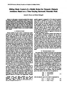
1 blank line (10-point font with single spacing) The chain of energy conversion adopted for the power supply of the DFIM consists of two converters, one on the stator and the other one on the rotor. A filter is placed between the two converters, as shown in figure1. 1 blank line (9-point font with single spacing) Stator

Rotor

PWM Inverters Load

Filter

Rectifiers 3 phase grid

DFIM

blank line (9-point font with single spacing) Figure 1. General scheme of DFIM drive installation 1 blank line (9-point font with single spacing)

The control strategy is determined from the DFIM model expressed in the (d,q) rotating reference frame. Figure 2 shows that the stator flux vector is oriented toward the direct axis (  s   sd and  sq  0 ) and it also rotates at  dq  d  dq / dt speed. The model is then expressed by (1). In steady state,  dq   s and  dq   s , and by imposing I to have a unitary power factor sd ref

1446 S.A. ARDJOUN at al. / IU-JEEE Vol. 12(1), (2012), 1445-1451

working [3]. And this model can be simplified and written in (4). So, we also obtain the null direct stator voltage component ( Vsd  0 ). 1 blank line (9-point font with single spacing)

11 blank line (10-point font with single spacing) The control of the DFIM vector is designed with an input/output current decoupling strategy which permits an independent control of the four current components, I sd , I sq , I rd and I rq . Concerning the details of this method,

they are presented in [4]. This decoupling strategy is based on state space DFIM modeling as in (6): 11 blank line (10-point font with single spacing)

 x  Ax  Bu   y  Cx

(6)

11 blank line (10-point font with single spacing) 1 blank line (9-point font with single spacing) Figure 2. Stator flux vector linked to the direct axis of the (d,q) frame 1 blank line (9-point font with single spacing)

General DFIM model 11 blank line (10-point font with single spacing) d  sd d s  Vsd (t )  R s I sd  dt  dt  sq  d  sq d s  Vsq (t )  R s I sq    sd  dt  dt  V (t )  R I  d  rd  d  r  r rd rq  rd dt dt  V (t )  R I  d  rq  d  r  rq r rq rd  dt dt 

T x [ I sd I sq I rd I rq ] R n

11 blank line (10-point font with single spacing) The state space vector, 11 blank line (10-point font with single spacing) T u  [V sd V sq V rd V rq ]  Rm

11 blank line (10-point font with single spacing) The input vector 11 blank line (10-point font with single spacing) (1)

T y  [ I sd I sq I rd I rq ]  R p

11 blank line (10-point font with single spacing) With n: state variables number, m: inputs number, p: outputs number. So, the different matrices of the state space equation are as below: 11 blank line (10-point font with single spacing)

11 blank line (10-point font with single spacing)

 sd   sq   rd   rq

A

 L s I sd  M sr I rd  L s I sq  M sr I rq  L r I rd  M sr I sd

(2)

 L r I rq  M sr I sq

s  r  

(3)

11 blank line (10-point font with single spacing) With  :angle between the stator and rotor winding,  s :angle between the stator winding and the axis d,

 b1 I 2  b3 I 2

0

 R r I rd  r  rq  R r I rq  r  rd

11 blank line (10-point font with single spacing) The electromagnetic torque is expressed by (5) 11 blank line (10-point font with single spacing) T em  N p M sr I sq I rd  N p  sd I sq (5)

With, I 2 

(4)

(7)

 b3 I 2



b2 I 2

(8)

The output matrix, 11 blank line (10-point font with single spacing)

Steady state DFIM model 11 blank line (10-point font with single spacing)  R s I sq  s  sd

 a2 I 2 



11 blank line (10-point font with single spacing) The control matrix, C  I 4

 r :angle between the rotor winding and the axis d.

Vsd  Vsq  Vrd V  rq

  j (s  )   

a3 I 2  j a5 

11 blank line (10-point font with single spacing) The dynamic matrix, 11 blank line (10-point font with single spacing) B

11 blank line (10-point font with single spacing)

 a1 I 2  j ( a  s )   a 4 I 2  j a6 

1 0

0

1 

,j

0  1

1 0 1 , I4   0 0  0 

0 0 0

1 0 0 0 1 0



0 0 0

11 blank line (10-point font with single spacing) Where: 11 blank line (10-point font with single spacing) a

1 

a5 



,a  1

M sr L

s

Rs L

,a  6

,a  2

s

M sr L

r

Rr L

,b  1

,a  3

r

1 L

R r M sr  L Lr s

,b  2 s

1 L

,a  4

,b  3 r

R s M sr  L Lr s

M sr L L s r

1447 S.A. ARDJOUN at al. / IU-JEEE Vol. 12(1), (2012), 1445-1451

And   (1 

2 M sr

Where )

e X

L s Lr

11 blank line (10-point font with single spacing) Consequently, the general scheme of applied decoupling current method is presented in figure 3. blank line (9-point font with single spacing)

blank line (9-point font with single spacing) Figure 3. Decoupling current feedback for DFIM blank line (9-point font with single spacing)

Ld  B  1 With  K d  B  1 A



n1 T

,X

d



And e - Error on the signal to be adjusted, λ - positive d

coefficient, n - system order, X - desired signal, X - state variable of the control signal. 1 blank line (10-point font with single spacing)  Convergence Condition 1 blank line (10-point font with single spacing) The convergence condition is defined by the equation Lyapunov [7], it makes the area attractive and invariant. 11 blank line (10-point font with single spacing) S(X)S(X)  0 (12) lank line (10-point font with single spacing)  Control Calculation 11 blank line (10-point font with single spacing) The control algorithm is defined by the relation 11 blank line (10-point font with single spacing) eq

u

n

(13)

Where u is the control vector, u (9)

1 blank line (10-point font with single spacing) The sliding mode control has been very successful in recent years. This is due to the simplicity of implementation and robustness against system uncertainties and external disturbances affecting the process. The basic idea of sliding mode control is first to draw the states of the system in an area properly selected, then design a law command that will always keep the system in this region [5]. The sliding mode control goes through three stages: 1 blank line (10-point font with single spacing)  Choice of Switching Surface 1 blank line (10-point font with single spacing) For a nonlinear system presented in the following form: 11 blank line (10-point font with single spacing) n (10) X  f(X,t) g(X,t)u(X, t); Χ   ,u   11 blank line (10-point font with single spacing) Where: f(X,t), g(X,t) are two continuous and uncertain non- linear functions, supposed limited. We take the form of general equation given by J.J.Slotine to determine the sliding surface given by [6]: 11 blank line (10-point font with single spacing) n 1

(11)



T d d d  x , x ,x , ...

11 blank line (10-point font with s

3. Sliding Mode Control

e



 X , X  x,x, ...,x

11 blank line (10-point font with single spacing)

uu

11 blank line (10-point font with single spacing) To obtain the decoupling current control the new input vector v is imposed [4], and it is associated with Stator Flux Oriented Vector Control (SFOVC) strategy. 1 blank line (10-point font with single spacing)

d  S( X)    λ   dt 

d

eq

is the equivalent

n

control vector, u is the switching part of the control (the correction factor) eq

can be obtained by considering the condition for the sliding regime, S(X, t)  0 .The equivalent control keeps the state variable on sliding surface, once they reach it. u

n u is needed to assure the convergence of the system

states to sliding surfaces in finite time. In order to alleviate the undesirable chattering phenomenon, J. J. Slotine proposed an approach to reduce it, by introducing a boundary layer of width  on either n

side of the switching surface [6]. Then, u is defined by 11 blank line (10-point font with single spacing) n

(14)  K sat( S ( X ) / ) 11 blank line (10-point font with single spacing) Where sat( S ( X ) / ) is the proposed saturation function,  is the boundary layer width, K is the controller gain designed from the Lyapunov stability Commonly, in DFIM control using sliding mode theory, the surfaces are chosen according to the error between the reference input signal and the measured signals [8,9]. 1 blank line (10-point font with single spacing) u

3.1. Speed Control 1 blank line (10-point font with single spacing) The speed error is defined by: 11 blank line (10-point font with single spacing) e  ref

(15)

11 blank line (10-point font with single spacing) For n =1, the speed control manifold equation can be obtained from equation (11) as follow: 11 blank line (10-point font with single spacing) S ( )  e    (16) ref

11 blank line (10-point font with single spacing)

1448 S.A. ARDJOUN at al. / IU-JEEE Vol. 12(1), (2012), 1445-1451

S ( )  

ref

 

(17)

obtain: 11 blank line (10-point font with single spacing)

11 blank line (10-point font with single spacing) With the mechanical equation: 11 blank line (10-point font with single spacing)   

N p M sr

ft

Cr ( I rq  ref   sd )  J t Ls Jt Jt

  1 M sr S  sd   ref  sd  sd   V sd  Ts I rd  Ts  

 

(18)

11 blank line (10-point font with single spacing) By replacing the mechanical equation in the equation of the switching surface, the derivative of the surface becomes: 11 blank line (10-point font with single spacing) S ( )  

ref

  

 

Cr f t  ( I rq  ref    (19) sd )  J t Ls J t J t 

N p M sr

11 blank line (10-point font with single spacing) We take: 11 blank line (10-point font with single spacing) ref eq n I rq  I rq  I rq

Substituting the expression of  sd in equation (24), we

11 blank line (10-point font with single spacing) The control current I rd is defined by: 11 blank line (10-point font with single spacing) ref eq n I rd  I rd  I rd

11 blank line (10-point font with single spacing) During the sliding mode and in permanent regime, we have: S ( sd )  0, S ( sd )  0, I n rd  0

 Ts 1 eq  ref I rd    sd  V sd   sd  Ts   M sr

11 blank line (10-point font with single spacing) During the sliding mode and in permanent regime, we have: 11 blank line (10-point font with single spacing)

11 blank line (10-point font with single spacing) Where, the correction factor is given by

S ( )  0, S ( )  0, I n rq  0

11 blank line (10-point font with single spacing) : positive constant. K

eq I rq  

J t Ls ref N p M sr  sd



Cr Jt



   Jt 

4. Simulation Results (21)

(22)

11 blank line (10-point font with single spacing) : positive constant. K I rq

1 blank line (10-point font with single spacing)

3.2. Stator Flux Control 1 blank line (10-point font with single spacing) In the proposed control, the manifold equation can be obtained by: 11 blank line (10-point font with single spacing) S ( sd )   ref sd   sd

(23)

11 blank line (10-point font with single spacing)  S ( sd )   ref sd   sd

(24)

11 blank line (10-point font with single spacing) With the flux equation 11 blank line (10-point font with single spacing) M

1

(29)

1 blank line (10-point font with single spacing)

11 blank line (10-point font with single spacing) Therefore, the correction factor is given by: 11 blank line (10-point font with single spacing) n I rq  K I sat( S ( )) rq

n I rd  K I sat( S ( sd )) rd

(28)

I rd

11 blank line (10-point font with single spacing) Where the equivalent control is: 11 blank line (10-point font with single spacing) ft

(27)

The equivalent control is: 11 blank line (10-point font with single spacing) (20)

    ref

(26)

sr (25)  sd  V sd  I   Ts rd T s sd 11 blank line (10-point font with single spacing)

1 blank line (10-point font with single spacing) To validate the robustness and good performance of speed and flux regulator in the sliding mode, we vary the speed and load torque with and without parameters uncertainties. Figure 4 shows a block diagram of the studied system The reference speed and torque are defined as follows: - t = 0 s: Flux installation, speed at zero - t = 0.25 s:: Motor start up with a speed reference of 157 rd/s - t = 1 s: Application of nominal constant torque. - t = 1.5 s: Changing direction of rotation - t = 2.5 s: Reversal of the torque In the case of parametric uncertainties, we limit our simulations for the worst case, that is to say, where the resistance is increasing by 50%, 30% of the inductances, inertia of 200% and friction of 500%. The simulations were performed using the MatlabSimulink software. The engine parameters are indicated in Annex. Figure 5 shows the response of the system without parametric uncertainties and figure 6 shows the response with parametric uncertainties. The simulation results clearly show that: The decoupling between the electromagnetic torque and stator flux is very satisfactory. In the transitory regime the current mark spikes without reaching the saturation, with increasing settling time in the case of parametric uncertainties, and in the steady state they remain at their nominal values.

1449 S.A. ARDJOUN at al. / IU-JEEE Vol. 12(1), (2012), 1445-1451

The speed response follows exactly the model applied with increasing response time in the case of parametric uncertainties and the impacts of load torque does not affect it. 1 blank line (10-point font with single spacing)

5. Conclusion 1 blank line (10-point font with single spacing) This paper suggests a sliding mode control method that is used for the speed and flux control of a double fed induction machine using stator flux vector oriented control with input-output decoupling. After modeling the system we have developed two controllers (one for the speed and the other one for the flux) using the sliding mode. With the appropriate choice of the parameters control and the smoothing of the discontinuity control, the chattering effects are reduced, and the torque fluctuations are decreased too. Simulation results have then shown robustness and good performances when the DFIM is confronted to internal and external perturbations. Furthermore, this regulation presents a simple robust control algorithm that has the advantage to be easily implantable in calculator.

6. Annex 1 blank line (10-point font with single spacing) Table 1. Nomenclature and numeric values 1 blank line (9-point font with single spacing)

Pn

1.5 kW

Nominal power

Usn

380 V

Stator nominal voltage

Urn

225 V

Rotor nominal voltage

Isn

4.3 A

Stator nominal current

Irn

4.5 A

Rotor nominal current

Np

2

Pair poles

Rs

1.75 Ω

Stator resistance

Rr

1.68 Ω

Rotor resistance

Ls

0.295 H

Stator inductance

Lr

0.104 H

Rotor inductance

Msr

0.165 H

Mutual inductance

Jt

0.0426 kg.m2 2 -1

Inertia

ft

0.00.27 kg.m .s

Friction

Ωn

1420 rpm

Nominal rotation speed

Figure 4. DFIM developed control

1450 S.A. ARDJOUN at al. / IU-JEEE Vol. 12(1), (2012), 1445-1451

40

Speed [rad/s]

Torque [N.m]

 ref

100

 0

-100

0

0.5

1

1.5

2

2.5

-40

3

30

10

20

Rotor currents [A]

15

5 0 -5

I

-10

I

-15

T

em

-20

T

r

0

Stator currents [A]

20

0

0.5

1

1.5

2

sd sq 2.5

0.5

1

1.5

2

2.5

3

2.5

3

Ird Irq

10 0 -10 -20

3

0

0

0.5

1

1.5

2

1.5

Rotor flux [Wb]

Stator flux [Wb]

0.8 1

 sd  sq

0.5

0

 rd

0.6 0.4

 rq

0.2 0 -0.2

0

0.5

1

1.5 Time [s]

2

2.5

3

0

0.5

1

1.5 Time [s]

2

2.5

3

2

2.5

3

Figure 5. The response of the system without parametric uncertainties

40

 ref 

Torque [N.m]

Speed [rad/s]

100

0

-100

20 0

Tem

-20

T

r

-40 0

0.5

1

1.5

2

2.5

3

0

0.5

1

1.5

20

Rotor currents [A]

Stator currents [A]

30

10 0 -10

Isd

-20

Isq

-30

0

0.5

40

I

20

I

rd rq

0 -20

1

1.5

2

2.5

3

0

0.5

1

1.5

2

2.5

3

0.8 1

Rotor flux [Wb]

Stator flux [Wb]

1.5

 sd  sq

0.5

 rd

0.6 0.4

 rq

0.2 0

0 0

0.5

1

1.5 Time [s]

2

2.5

3

-0.2

0

0.5

1

1.5 Time [s]

2

2.5

Figure 6. The response of the system with parametric uncertainties (R+50%, L+30%, Jt+200%, and ft +500%)

3

1451 S.A. ARDJOUN at al. / IU-JEEE Vol. 12(1), (2012), 1445-1451

7. References 1 blank line (10-point font with single spacing) [1] P-E. Vidal, and M. Pietrzak-david, “Flux Sliding Mode Control of a Doubly Fed Induction Machine”, European Conference on Power Electronics and Applications, 2005. [2] G. Salloum, R. Mbayed, and M. Pietrzak-david, “Mixed Sensitivity H∞ Control of Doubly Fed Induction Motor”, IEEE International Symposium on Industrial Electronics, pp: 1300 - 1304, 2007. [3] M. Abdellatif, M. Pietrzak-David and I. Slama-Belkhodja, “Sensitivity of the Currents Input-Output Decoupling Vector Control of the DFIM versus Current Sensors Fault”, 13th International Power Electronics and Motion Control Conference, EPE-PEMC, pp 938-944, 2008. [4] G. Salloum, “Contribution à la commande robuste de la machine asynchrone à double Alimentation", Thèse de Doctorat en Génie Électrique, Institut National Polytechnique deToulouse, France, 2007. [5] P-E. Vidal, "Commande non-linéaire d'une machine asynchrone à double alimentation", Thèse de doctorat en Génie Electrique, Institut National Polytechnique de Toulouse, France, 2004. [6] J.J.E. Slotine, W. Li, “Applied nonlinear control”, Prence Hall, USA, 1998. [7] P. Lopez and A. S. Nouri, "Théorie Elémentaire Et Pratique de La Commande Par Les Régimes Glissants", Springer, 2006. [8] V. I. Utkin, “Sliding mode control design principles and applications to electric drives”, IEEE Trans. Ind. electronic, vol. 40, pp.23-36, Feb.1993. [9] V.I. Utkin, “Variable structure systems with sliding modes”, IEEE Trans. Automat. Contr., vol. AC-22, no. 2. pp. 212-222, Apr.1977.

1 blank line (10-point font with single spacing)

Biographies 1 blank line (10-point font with single spacing) Sid ahmed El Mahdi ARDJOUN was born in 1985 in Sidi Bel Abbes, Algeria. He received his BS and MS degree in electrical engineering from the Electrical Engineering Institute of The University of Sidi Bel Abbes in 2008 and 2010 respectively. Currently he is working on his PhD thesis. His main areas of research interests are control of electric drives (robust and intelligent control) in renewable energy domain. Mohamed ABID was born on 11.02.1963. In 1997 he graduated (MSc) with distinction at the department of electrical engineering of the faculty of science engineering at Djillali Liabes University in Sidi Bel Abbes, Algeria. He defended his PhD in the field of electrical engineering in 2005; his thesis title was “The optimized control adaptation to the field-oriented induction machine fed by a PWM converter”. Since 2000 he is teaching at the department of electrical engineering at Djillali Liabes University in Sidi Bel Abbes, Algeria. His scientific research is focusing on Modeling and Simulation of electric machines, Sliding mode in continuous systems, Control of electric drives. Abdelghani AISSAOUI was born on 07.10.1967. In 1997 he graduated (MSc) with distinction at the department of electrical engineering of the faculty of science engineering at Djillali Liabes University in Sidi Bel Abbes, Algeria. He defended his PhD in the field of electrical engineering in 2007; his thesis title was “Neural network and fuzzy logic used to control a synchronous machine”. Since 2001 he is teaching at the department of electrical engineering at the University of Bechar, Algeria. His scientific research is focusing on Power electronics and Control of electrical machines. Ahmed Tahour was born in 1972 in ouled mimoun, Tlemcen, Algeria. He received his BS degree in electrical engineering from the Electrical Engineering Institute of The University of Sidi Bel Abbes in 1996, and the MS degree from the Electrical Engineering Institute of The University of Sidi Bel Abbes in 1999 and The PhD from the Electrical Engineering Institute of the University of Sidi Bel Abbes in 2007. He is currently Professor of electrical engineering at University of Bechar (Algeria). His current research interest includes power electronics and control of electrical machines.