A Rule-Based and Imperative Language for Biochemical Modeling

A Rule-Based and Imperative Language for Biochemical Modeling and Simulation Ðurica Nikoli´c1,2 , Corrado Priami1,3 , and Roberto Zunino1,3 1

The Microsoft Research - University of Trento Centre for Computational and Systems Biology 2 University of Verona, Italy 3 University of Trento, Italy

Abstract. We present COSBI LAB Language (L for short), a simple modeling language for biochemical systems. L features stochastic multiset rewriting, defined in part through rewriting rules, and in part through imperative code. We provide a continuous-time Markov chain semantics for L at three different abstraction levels, linked by Galois connections. We then describe a simulation algorithm for the most concrete semantics, which is then adapted to work at higher abstract levels while improving space and time performance. Doing so results in the well-known Gillespie’s Direct Method, as well as in a further optimized algorithm.

1 Introduction In this paper we present a computer language, called L , for modeling and simulating biochemical systems. In such setting, we are concerned with the modeling of the kinds of behaviour leading to the creation of biomolecular complexes and their mutual interaction. Complexes are to be thought as an aggregation of smaller molecules, kept together by chemical bonds on specific zones called interaction sites. Different kinds of mathematical structures have been used to model such entities. Often, these take inspiration from graphs and their generalizations, e.g., hypergraphs. Here, the smaller molecules are represented by graph nodes, which are taken as primitive stateful entities. We shall name these stateful nodes “boxes”. Boxes also have a list of sites, from which they can be connected to other boxes by (undirected) edges. In this framework, complexes are just the connected components of the graphs. System evolution is then typically modeled via a stochastic transition system, hence providing a semantics based on continuous-time Markov chains; this is done to capture the inherent uncertainty of the biological phenomena, which are “noisy” in their nature. The actual definition of the transition system depends on the modeling language at hand. For instance, BlenX [5] is a language which uses a graph-like representation of complexes, whose boxes are equipped with a process in a stochastic process algebra. There, the stochastic operational semantics of the processes inside the boxes form the basis for defining the transition system for graphs. Kappa [2] instead resorts to stochastic rewriting rules, borrowing from graph rewriting techniques. These rules can be used to express in an intuitive way how the graph is affected by biochemical reactions. Often, however, the precise graph structure of complexes, their chemical bonds, and the nature of the interaction sites is still unknown to researchers in biology. Modelers G. Eleftherakis, M. Hinchey, and M. Holcombe (Eds.): SEFM 2012, LNCS 7504, pp. 16–32, 2012. c Springer-Verlag Berlin Heidelberg 2012 

A Rule-Based and Imperative Language for Biochemical Modeling and Simulation

17

wishing to use graph-based modeling languages are then asked to provide more data than those available. In such cases, it would be better to use a less detailed structure to represent complexes. In our L language we use box multisets in lieu of box graphs. Consequently, interaction sites are no longer represented, as well as exact chemical bonds. Rather, we just represent the fact that two molecules belong to the same complexes (or to different ones). This approach seem to be closer to the actual knowledge available to researchers. As a bonus, we also get some performance improvements in simulation, since e.g. graph isomorphism tests (untractable, but quadratic time under certain assumptions [7]) are now replaced by multiset equality tests (linear time with most representations). In L , we use stochastic multiset rewriting rules to define the evolution of a system. Three kind of rules are used: association rules (assoc) which merge two complexes, dissociation rules (dissoc) which split them, and general dynamics dyn to model the rest of the interactions. These rules are defined using complex patterns, selecting which complexes are to be rewritten. Rewriting is, in part, automatic (for assoc and dissoc) and can be augmented by imperative code whenever one needs to describe custom multiset manipulations. The effect of this code is atomic: no other rule firing is interleaved. Having atomic “large” effects is useful, since otherwise such effects need to be carefully programmed across many rules, often using “infinite” stochastic rates and dealing with all the resulting concurrency issues [6]. For instance, if we want to model a vescicle releasing at once all its carried molecules (the number of which is not statically known), we can not use a basic rule, yet it is straightforward to program this behaviour. We present the syntax of L in Sect. 2, and its semantics in Sect. 3. We then study how the language can be efficiently simulated. In order to do so, we apply abstract interpretation and construct two more abstract semantics in Sect. 4. We then apply this to construct efficient simulation algorithms for L in Sect. 5. We start from a simple, yet inefficient algorithm which is then adapted to exploit the abstract semantics. This results in improvements to space and time performance. The algorithms constructed in this way are the well-known Gillespie’s Direct Method [4] as well as a new improvement of it which better takes advantage of the features of L .

2 Syntax In Figure 1 we show the syntax of the L language. We give a short comment on the constructs in that figure. BasicT ype stands for a primitive type used in our language, while BasicLiteral ranges over their values. The modeler can declare a box type, by specifying a name for it and of a set of fields having basic types. More formally, FieldDecl is a sequence of field declarations of form Field : BasicT ype, where Field is the name of the field, and is unique inside the box. The field list can be empty (). Then, the declaration of a box type BoxDecl has the form BoxT ype{FieldDecl}, where BoxT ype is a name for the declared type. Moreover, FieldInit is a (possibly empty) sequence of initialized fields, while BoxLiteral represents a box having all its declared fields instantiated. For example, A{x : int; y : real} is a declaration of a box type A containing fields x and y of the given types, and A{x = 3; y = 1.0} is an instantiation. We use Box to denote the set of all possible box instantiations.

18

Ð. Nikoli´c, C. Priami, and R. Zunino BasicT ype BasicLiteral Field FieldDecl FieldInit Exp

BoxT ype BoxDecl BoxLiteral C plxLiteral C plxLiteralT ail Complexes ComplexesT ail Pattern PatternT ail Assoc Dissoc Dyn Block CmdBlock Cmd BoxCommand

Decl Run Model

::= bool | int | real ::= BoolLiteral | IntLiteral | RealLiteral ::= Ide ::=  | Field : BasicT ype; FieldDecl ::=  | Field = BasicLiteral; FieldInit ::= BasicLiteral | null | Ide | Exp ∧ Exp | ¬Exp | Exp + Exp | Exp − Exp | Exp ∗ Exp | Exp = Exp | Exp < Exp | Exp.Field | Exp.count(BoxT ype) | Exp.first(BoxT ype) ::= Ide ::= BoxT ype{FieldDecl} ::= BoxT ype{FieldInit} NOTE: all declared fields must be instantiated ::= [IntLiteral : BoxLiteral; C plxLiteralT ail] ::=  | IntLiteral : BoxLiteral; C plxLiteralT ail ::= IntLiteral : C plxLiteral; ComplexesT ail ::=  | IntLiteral : C plxLiteral; ComplexesT ail ::= [BoxT ype{FieldInit} PatternT ail] ::=  | , BasePattern ::= assoc Pattern Pattern rate Exp react Block ::= dissoc Pattern Patternno∗ rate Exp react Block ::= dyn Pattern1 . . . Patternn rate Exp react Block ::= var Ide := Exp; Block | CmdBlock ::= end | Cmd ; CmdBlock ::= skip | Ide := Exp | if Exp then Block else Block | while Exp do Block | BoxCommand ::= Ide := Exp.spawn(BoxLiteral, . . .) | Exp.spawn(Exp) | Exp.remove(Exp) | Exp.merge(Exp) | Exp.move(Exp, Exp) | foreach Ide : BoxT ype in Exp do Block | Exp.Ide := Exp ::= Assoc | Dissoc | Dyn | BoxDecl ::= run Complexes end ::= Run | Decl; Model

Fig. 1. Syntax of the L language

For any set S, we write mset S for the set of multisets over S, which we sometimes identify with the set of functions S → N. A complex is a multiset of boxes, which we represent in our syntax by a C plxLiteral. The latter is a non-empty sequence of the form IntLiteral : BoxLiteral, where IntLiteral denotes how many instances of BoxLiteral are present in the complex. When IntLiteral = 1, we omit to write it. For instance, [2 : A{x = 3; y = 1.0}, B{}] is a complex. We use Cplx = mset Box to denote the set of all possible complexes. The whole system state is then defined via the Run clause, which specifies an initial sequence of Complexes, having form IntLiteral : C plxLiteral where IntLiteral represents the initial population of the complex in the system at hand. The dynamics of the system is given by multiset rewriting rules, which continuously modify the system at hand (if no rule applies, the system does not evolve further). Our rules are based on complex patterns. A Pattern is a sequence of literals of form BoxT ype{FieldInit}, possibly followed by a wildcard ∗. Intuitively, a pattern without ∗ matches with complexes having exactly the specified boxes, while the wildcard allows matching with complexes including other boxes as well. More formally, we say that a box B1 { f1 = v1 , . . . , fn = vn } matches with a box B2 {g1 = h1 , . . . , gm = hm } if B1 = B2 ,

A Rule-Based and Imperative Language for Biochemical Modeling and Simulation

19

n ≤ m and for each i ∈ [1..n] there exists j ∈ [1..m] such that fi = g j and vi = h j . Then, we say that a complex c ∈ Cplx matches with a pattern p, denoted with c |= p, if one of the following conditions holds: – p does not end with ∗, and there is a bijective correspondence between boxes in p and those in c, where correspondent boxes match. – p does end with ∗, and there is an injective correspondence between boxes in p and those in c, where correspondent boxes match. The following example illustrates some pattern matchings. Example 1. Consider complexes c1 = [A{x = 1}], c2 = [B{}], c3 = [A{x = 0}, A{x = 1}], c4 = [A{x = 1}, B{}] and c5 = [A{x = 1, y = 4}] and patterns p1 = [A], p2 = [A, A], p3 = [A, ∗], p4 = [B], p5 = [B, ∗] and p6 = [A{x = 1}]. Then, only the following relations hold: c1 |= p1 , c1 |= p3 , c1 |= p6 , c2 |= p4 , c2 |= p5 , c3 |= p2 , c3 |= p3 , c4 |= p3 , c4 |= p5 , c5 |= p1 , c5 |= p3 , c5 |= p6 .  Having defined patterns, we can now discuss the rewriting rules which lead the evolution of the system. Our language features three kinds of such rules, namely Assoc, Dissoc and Dyn. A rule assoc p1 p2 rate Exp react Block allows pairs of complexes matching with p1 and p2 to associate. When that happens, the two reactant complexes merge their boxes and form a new larger complex, mimicking the association of two macromolecules in biological systems. The rate expression Exp provides the rate for the stochastic transition, thus defining the “speed” of the association. The rate expression is allowed to inspect the boxes in the two reactants via two special variables reactant1 and reactant2. For instance, assoc [A] [B, ∗] rate 5.2 ∗ reactant1 .first(A).mass defines a rate proportional to the mass of the first reactant. When an assoc rule is fired, after the complexes are associated the code block specified in the react part is run. This can access the newly formed product (via a special product variable) and modify it further, e.g. by changing box fields, or adding/removing boxes. The react code block can also spawn entirely new complexes. A rule dissoc p1 p2 rate Exp react Block specifices the dual operation, namely dissociation of a complex into two subcomplexes. Here, p1 specifies the complex to break up, while p2 matches with a subcomplex to separate (no wildcard ∗ is allowed in p2 ). The rate expression Exp can access reactant1 to provide a dissociation stochastic rate, which is intended to define how fast is the reactant to split. In the case p2 has multiple matches inside the reactant, we let all of them define an equally probable dissociation, hence effectively dividing the rate among all the possible splits. After the rule triggers and the split is performed, the react code block is run, and can access the new complexes using the variables product1 and product2. Rule dyn is used to define a generic molecular dynamics. Its semantics is as for assoc, except that no complex merge is performed, and the react code block still has access to the unmerged complexes reactant1 and reactant2. This rule effectively subsumes assoc and dissoc, in that association/dissociation can be programmed manually in the code block. However, associations and dissocations are so common to deserve a special construct. Instead, the typical use for dyn is the modeling of monomolecular reactions, in which only one reactant is present.

20

Ð. Nikoli´c, C. Priami, and R. Zunino

The code blocks in rules are written in an imperative language, the constructs of which are mostly standard. Therefore, we just briefly discuss the more peculiar ones. Since the state of L is stored in complexes, i.e. in multisets of boxes, we need constructs to inspect and modify those. We provide a way to loop over all the boxes of a given type in a complex (foreach b : BoxT ype in complex). To precisely define the semantics of such loop, we require that the visit order follows the lexicographic order of box values. The expression complex.first(BoxT ype) returns the first box in such ordering. Further commands allows one to add (complex.spawn) and remove (complex.remove) boxes in a complex. Similar operations can be done at the complex level: new complexes can be created, and existing ones removed. We provide also ways to move boxes between complexes (move) as well as to merge two complex as it happens for association (merge). Example 2. As a simple example, we provide an L model for the enzymatic reaction shown below: k1 k3 k2 −−−  E+S  − ES −→ EI −→ E + P k−1

The first double arrow models an enzyme molecule (E) associating and dissociating to a substrate molecule (S ). When associated, the complex ES can react (second arrow): the enzyme changes the substrate into some intermediate molecule (I). This reaction is not reversible. Then, the intermediate molecule can dissociate from the enzyme, which releases a product (P) in the system (third arrow). In L , we can model this behaviour as follows. Below, the react blocks are used to change S into I, and then I into P. E{}

S {}

I{}

P{}

assoc [E] [S ] rate k1 ; dissoc [E, S ] [S ] rate k−1 ; dyn [E, S ] rate k2 react reactant1 .remove(reactant1 .first(S )); reactant1 .spawn(I{}); end; dissoc [E, I] [I] rate k3 react product2 .remove(product2 .first(I)); product2 .spawn(P{}); end; run 100 : [E]; 100 : [S ]; end



3 Semantics In this section we provide a semantics for the rules of our L language. To keep our presentation short, we focus on the semantics of the assoc rule, only. The formal semantics of the dissoc and dyn rules can be indeed defined similarly. Suppose we are given a set of complexes annotated with their names. Names uniquely identify the instances of complexes present in the system, so that complexes comprised by exactly the same boxes are still distinguishable. For the sake of simplicity, we assume that complexes’ names are natural numbers. Then, suppose that we are

A Rule-Based and Imperative Language for Biochemical Modeling and Simulation

21

given an assoc rule which states that all the pairs of complexes satisfying patterns p1 and p2 react with a stochastic rate specified by an expression e. The semantics of the assoc rule then collects the stochastic transitions involving all such pairs of complexes, and their corresponding rates. We start by defining two auxiliary binary set operators, which are similar to the cartesian product. Operator ⊗ defines the set of unordered pairs ({x1 , x2 }), while operator ⊗ˆ defines the set of unordered pairs of distinct elements (hence requiring x1  x2 ). ˆ Given two arbitrary sets S1 and S2 , we define Definition 1 (⊗ and ⊗). S1 ⊗ S2 = {{x1 , x2 } | x1 ∈ S1 ∧ x2 ∈ S2 }

ˆ S2 = {{x1 , x2 } | x1 ∈ S1 ∧ x2 ∈ S2 ∧ x1  x2 }. S1 ⊗

The following definition introduces the notion of system, representing a set of complexes enriched with their names, and the notion of transition, representing two different complexes that can react with a certain rate. Definition 2 (Systems and Transitions). A system σ is a set of annotated complexes, i.e., ordered pairs n, c ∈ N × Cplx, where c and n represent a complex and its unique name, respectively. We write Sys0 = ℘(N × Cplx) to denote the set of all the possible systems. A transition is an ordered pair whose first element determines the reactants, while the second element is the rate of the reaction. The reactants are characterized by ˆ Cplx))×R+ an unordered pair of annotated complexes. We write Tr0 = ((N× Cplx)⊗(N× to denote the set of all possible transitions. Moreover, we let Res0 = ℘(Tr0 ). It is worth noting that Res0 denotes all possible sets of transitions, and therefore represents the set of all possible semantics of an assoc rule. Example 3. Let c1 = [A{x = 0}], c2 = [A{x = 1}] and c3 = [B] be three complexes, and suppose that a system σ is composed of 2, 1 and 2 instances of c1 , c2 and c3 respectively. Then, we represent σ as follows: σ = { 0, c1 , 1, c1 , 0, c2 , 0, c3 , 1, c3 }. If we suppose that 0, c1 and 0, c2 can react with a rate 1.0, the corresponding transition is given as: { 0, c1 , 0, c2 }, 1.0 .  We now define a function which selects from a system only those annotated complexes which match with a given pattern. Definition 3. Given a pattern p, we define a map p0 : Sys0 → Sys0 called the evaluation of p in Sys0 as: p0 σ = { n, c ∈ σ | c |= p}, for any σ ∈ Sys0 . Example 4. Consider the system σ defined in Example 3 and a pattern [A] denoting the complexes composed of only one box whose its type is A. Since complexes c1 and c2 match with [A], while c3 does not, we have [A]0 σ = { 0, c1 , 1, c1 , 0, c2 }.  We now define to the actual semantics of the assoc rule. Its general form is the following: assoc p1 p2 rate e react Block. Starting from a system σ , we evaluate patterns p1 and p2 (Definition 3), obtaining two systems σ1 and σ2 whose complexes match with patterns p1 and p2 respectively. Our goal is to determine all possible transitions whose first reactant belongs to σ1 , and the second one belongs to σ2 . The rate of each

22

Ð. Nikoli´c, C. Priami, and R. Zunino

transition is determined by evaluating the expression e. This evaluation depends on an environment, i.e., a function which maps special variables reactant1 and reactant2 to their values. These values are the complexes which take part in the transition. The following definition explains how it is possible to evaluate the rate characterized by an expression e of a reaction between two complexes c1 and c2 . It is worth noting that the rate expression e should be “symmetric” in reactant1 and reactant2 : swapping their values should not affect the resulting association rate. This reflect the fact that in biology association happens between unordered complex pairs. To stress and enforce this symmetry, below we compute the rate as the average of the rates resulting from both orders. Definition 4. Let c1 and c2 be two complexes and let e be an expression characterizing the rate of the reaction between these complexes. We determine the rate of this reaction as follows: eexp ρ1 + eexp ρ2 , rate(c1 , c2 , e) = 2 where ρ1 = [reactant1 → c1 , reactant2 → c2 ] and ρ2 = [reactant1 → c2 , reactant2 → c1 ]. Given an assoc rule and a system, we define the set of all possible transitions that can occur between complexes of the system. Definition 5 (Semantics of assoc). Consider a rule assoc p1 p2 rate e react B and a −nc state σ ∈ Sys0 . We define the map p1 , p2 , eassoc : Sys0 → Res0 as 0 −nc  σ = p1 , p2 , eassoc 0   { n1 , c1 , n2 , c2 }, rate(c1 , c2 , e) ∈ Tr0 | n1 , c1 ∈ p1 0 σ ∧ n2 , c2 ∈ p2 0 σ .

: ℘(Sys0 ) → ℘(Res0 ) is defined as follows: The collecting semantics p1 , p2 , eassoc 0   assoc  assoc−nc  σ | σ ∈ Σ  . p1 , p2 , e0 Σ = p1 , p2 , e0 Note that the semantics of the assoc rule contains only transitions of type Tr0 , i.e., the ones in which reactants must be different. This does not prevent two identical complexes to react, since they have different names. However, a complex is prevented to react with itself, which would be unwanted. Example 5. Let us consider, one more time, the system σ defined in Example 3 and let us determine the semantics of the rules rule1 : assoc [A] [B] rate 1.0

rule2 : assoc [A] [A] rate 1.0.

In Example 4 we showed that [A]0 σ = { 0, c1 , 1, c1 , 0, c2 }. We can, similarly show that [B]0σ = { 0, c3 , 1, c3 }. The following table represents the semantics of the rules: rule1 gives rise to transitions 1.-6. from the following table, while rule2 gives rise to transitions 7.-9. 1. { 0, c1 , 0, c3 }, 1 2. { 0, c1 , 1, c3 }, 1 3. { 1, c1 , 0, c3 }, 1

4. { 1, c1 , 1, c3 }, 1 5. { 0, c2 , 0, c3 }, 1 6. { 0, c2 , 1, c3 }, 1

rule2 7. { 0, c1 , 0, c2 }, 1 8. { 1, c1 , 0, c2 }, 1 9. { 0, c1 , 1, c1 }, 1

rule1

Transitions 1.-6. occur between a complex matching with [A] and a complex matching with [B] and their rate is 1, while in transitions 7.-9. both complexes match with [A]. 

A Rule-Based and Imperative Language for Biochemical Modeling and Simulation

℘(Sys0)

[p1 ], [p2 ], eassoc 0

α1sys γ1sys Sys1 = Sys2

℘(Sys1) ℘(Sys2)

23

℘(Res0) α1res γ1res

[p1 ], [p2 ], eassoc 1

℘(Res1) α2res γ2res

[p1 ], [p2 ], eassoc 2

℘(Res2)

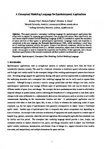
Fig. 2. Relationships between different levels of abstraction

Below, we state a simple property of the semantics of our expressions and commands. As it happens in nominal calculi and in most languages with references, we have that the actual names (n) used to annotate the “objects” (the complexes n, c ) are immaterial. Lemma 1. The semantics of expressions, commands, and rewriting rules are stable w.r.t. the renaming of annotated complexes. In particular, renaming does not affect the computed transition rates for rules, or their modifications of the state.

4 Abstraction There might be a huge number of annotated complexes satisfying the two patterns specified by an assoc rule that react. Hence, the number of reactions they give rise can becomes enormous. Although precise, the provided semantics for rules can lead to an inefficient simulation, as we will see. In this section we define two levels of abstraction which we shall exploit to perform some optimization in the simulation of L models. We call the actual semantics of the assoc rules defined in Section 3 the semantics of level 0, while we refer to our new abstraction levels as level 1 and level 2. For both of them, we define some opportune abstractions of Sys0 (Sys1 and Sys2 ) and Res0 (Res1 and Res2 ), show how they can be related (via pairs of functions α sys−γ sys and αres−γres ) and define two abstract semantics (p1 , p2 , eassoc and p1 , p2 , eassoc ) representing a sound 1 2 of the assoc rules. In Figure 2 approximation of the actual semantics p1 , p2 , eassoc 0 we give a brief outline of this idea which we then formalize in Sections 4.1 and 4.2. 4.1 Abstraction at Level 1 In Section 3 we have stated that the information about complexes’ names is not relevant for the actual semantics of the assoc rules. Therefore, it is possible to abstract away this piece of information and define another, more abstract semantics of these rules. In the following we will define counterparts of Definitions 2, 3 and 5. Although the names of complexes are not relevant for the computation of reaction rates, it is important to know the exact amount of each complex present in a system,

24

Ð. Nikoli´c, C. Priami, and R. Zunino

i.e. its population. This fact gives rise to another definition of the notion of system, on a different level of abstraction. More precisely, for each complex, we memorize the number of instances of that complex present in a system. Then we remove information about complexes’ names from the definition of transitions as well. The following definition formalizes these intuitions. Definition 6. A system σ is a multiset of complexes, i.e., σ ∈ mset Cplx = Sys1 . A transition is an ordered pair whose first element determines the set of reactants, while the second element is the rate of the reaction. The set of reactants can be composed of 1 or 2 elements. The former case occurs when two identical complexes react, while the latter case occurs when the reactants are not identical. We write Tr1 = (Cplx⊗Cplx)×R+ to denote the set of all possible transitions. Moreover, we let Res1 = ℘(Tr1 ). Example 6. Under the hypotheses of Example 3 regarding the structure of complexes c1 , c2 and c3 and their populations which are, respectively 2, 1 and 2, we define the state σ = [c1 → 2, c2 → 1, c3 → 2].  Definition 7. We define a function function names : Cplx × Sys0 → ℘(N) which for every complex c ∈ Cplx and every system σ ∈ Sys0 returns all possible names that c might have in σ as names(c, σ ) = {n ∈ N | n, c ∈ σ }.     It is worth noting that ℘(Sys0 ), ⊆, ∪, ∩, ∅, Sys0 , and ℘(Sys1 ), ⊆, ∪, ∩, ∅, Sys1 (or     shortly, ℘(Sys0 ), ⊆ and ℘(Sys1 ), ⊆ ) are complete lattices. In the following we show that they are also related by a Galois connection [1]. Definition 8. Let β1sys : Sys0 → Sys1 be defined as β1sys (σ ) = λc. |names(c, σ )|. We define the abstraction map α1sys : ℘(Sys0 ) → ℘(Sys1 ) and the concretization map sys γ1 : ℘(Sys1 ) → ℘(Sys0 ) as: α1sys (Σ  ) = {β1sys (σ ) | σ ∈ Σ  } Lemma 2.



γ1sys (Σ) =



{Σ  | α1sys (Σ  ) ⊆ Σ}.

 sys sys   ℘(Sys0 ), ⊆ , α1 , γ1 , ℘(Sys1 ), ⊆ is a Galois connection.

The abstraction map α1 modifies a system σ by substituting the names of the complexes belonging to that system with their population. The definition of γ1sys depends on α1sys and derives from a well-known result from the theory of abstract interpretation. Its meaning is clarified by the following lemma. sys

sys

Lemma 3. Let δ1 : Sys1 → ℘(Sys0 ) be a function defined as: δ1sys(σ) = {σ ∈ Sys0 | ∀c ∈ Cplx. |names(c, σ )| = σ(c)}. sys

Then, γ1 (Σ) =



σ∈Σ

sys

δ1 (σ).

In the following we perform a similar abstraction to the set of transitions Res0 by removing all pieces of information regarding the names of the complexes that can react. At this point, it might be the case that more than one transition has the same reactants. We group all these transitions together and we assign them a rate obtained as sum of

A Rule-Based and Imperative Language for Biochemical Modeling and Simulation

25

the rates of each single transition. For instance, consider the transitions 5. and 6. from Example 5: { 0, c2 , 0, c3 }, 1 , { 0, c2 , 1, c3 }, 1 ∈ Tr0 . By removing complexes’ names, we have two transitions of the same form: {c2 , c3 }, 1 . The idea is then to substitute them with only one transition with rate 1+1 = 2: {c2 , c3 }, 2 ∈ Tr1 . This rate is called propensity. We formalize our idea: the map comp we define below substitutes the reactants of each transition by the set composed of their complexes, while the map prop calculates the propensities of new transitions in the way we hinted at above. Definition 9. We define maps comp : Res0 → ℘(Cplx ⊗ Cplx) and prop : (Res0 × (Cplx ⊗ Cplx)) → R as: comp(R ) = {{c1 , c2 } | ∃n1 , n2 ∈ N.∃r ∈ R+ . { n1 , c1 , n2 , c2 }, r ∈ R } prop(R , A) = B,r ∈R s.t. comp({ B,r })=A r

Example 7. Let R be the set composed of the 9 transitions obtained in Example 5. Then, comp(R ) = {{c1 }, {c1 , c2 }, {c1 , c3 }, {c2 , c3 }}. On the other hand, the propensities are prop(R , {c1 }) = 1, prop(R , {c1 , c2 }) = prop(R , {c2 , c3 }) = 2, prop(R , {c1 , c3 }) = 4 and prop(R , A) = 0 for all other A ∈ ℘(Cplx ⊗ Cplx).  We can now define another pair of abstraction and concretization maps in order to relate Res0 and Res1 .

Definition 10. We define the abstraction map αres 1 : ℘(Res0 ) → ℘(Res1 ) and the concretization map γ1res : ℘(Res1 ) → ℘(Res0 ) as:    αres A, prop(R , A) | A ∈ comp(R )} | R ∈ R } 1 (R ) = {{   γ1res (R) = {R | αres 1 (R ) ⊆ R}.   res Lemma 4. ℘(Res0 ), ⊆ , αres 1 , γ1 , ℘(Res1 ), ⊆ is a Galois connection. We define a map which removes from a system σ ∈ Sys1 corresponding to a multiset of complexes (Definition 6) all those complexes not matching with a given pattern. Definition 11. Given a pattern p and a system σ ∈ Sys1 , the evaluation of p in σ is a map p1 : Sys1 → Sys1 defined as: ⎧ ⎪ ⎪ ⎨σ(c) p σ = λc. ⎪ ⎪ ⎩0 1

if c |= p otherwise.

Example 8. Consider the system σ defined in Example 6 and a pattern [A]. Since c1 and c2 match with p, while c3 does not, we have [A]1σ = [c1 → 2, c2 → 1, c3 → 0].  Given a system σ ∈ Sys1 , two complexes in it that may react, and the rate expression specified by an assoc rule, the following definition specifies how the propensity of all possible transitions induced by σ which have these complexes as reactants is computed.

26

Ð. Nikoli´c, C. Priami, and R. Zunino

Definition 12. Let c1 and c2 be two complexes appearing in a system σ ∈ Sys1 and let e be an expression characterizing the rate of the reaction between these complexes. We determine the propensity of this reaction as follows: pσ (c1 , c2 , e) =

σ(c) · (σ(c)−1) · eρ1 2

pσ (c1 , c2 , e) = σ(c1 ) · σ(c2 ) ·

eρ2 +eρ3 , 2

where the first equation applies when c1 = c2 = c, otherwise the second applies; also, above we let ρ1 = [reactant1 → c, reactant2 → c], ρ2 = [reactant1 → c1 , reactant2 → c2 ] and ρ3 = [reactant1 → c2 , reactant2 → c1 ]. In the following we define p1 , p2 , eassoc , the abstract semantics at level 1 of the actual 1 semantics of the assoc rules (Definition 5). Definition 13 (Level 1 semantics of assoc). Consider a state σ ∈ Sys1 and a rule −nc assoc p1 p2 rate e react B. We define the map p1 , p2 , eassoc : Sys1 → Res1 as 1 −nc p1 , p2 , eassoc σ = { {c1 , c2 }, pσ (c1 , c2 , e) ∈ Tr1 | p1 1 σ(c1 )  0 ∧ p2 1 σ(c2 )  0}. 1

The collecting semantics p1 , p2 , eassoc : ℘(Sys1 ) → ℘(Res1 ) is defined as follows: 1 assoc−nc p1 , p2 , eassoc Σ = {p , p , e σ | σ ∈ Σ}. 1 2 1 1 Example 9. Let us consider, one more time, rule1 and rule2 introduced in Example 5 and the system σ defined in Example 6. Let us determine the semantics at level 1 of these rules in σ. In Example 8 we showed that [A]1 σ = [c1 → 2, c2 → 1, c3 → 0]. We can, similarly show that [B]1σ = [c1 → 0, c2 → 0, c3 → 2]. By Definition 12, we have: pσ (c1 , c3 , 1) = 4 pσ (c2 , c3 ) = 2 pσ (c1 , c2 , 1) = 2 pσ (c1 , c1 ) = 1 pσ (c2 , c2 ) = 0. The following table represents the semantics at level 1 of our rules: rule1 gives rise to transitions 1.-2., while rule2 gives rise to transitions 3.-4. rule1 1. {c1 , c3 }, 4 2. {c2 , c3 }, 2

rule2 3. {c1 }, 1

4. {c1 , c2 }, 2

It is worth noting that since pσ (c2 , c2 ) = 0, transition {c2 }, pσ (c2 , c2 ) does not belong −nc to Tr1 , and therefore cannot be in [A], [A], eassoc .  1 The following lemma shows a relationship between the semantics at levels 0 and 1. Lemma 5. Given an expression e and two patterns p1 and p2 , the following condition holds: sys assoc p1 , p2 , eassoc = αres ◦ γ1 . 1 ◦ p1 , p2 , e0 1 4.2 Abstraction at Level 2 In this section we propose an additional abstraction of Res1 which calculates the cumulative propensity of all the reactions the assoc rule gives rise to. Abstraction of systems is the same one we introduced in the previous subsection.

A Rule-Based and Imperative Language for Biochemical Modeling and Simulation

27

Definition 14. A system σ is as a multiset of complexes, i.e., σ ∈ Sys2 = Sys1 = mset Cplx. Moreover, we let Res2 = R. We shall sometimes write σ instead of σ# to stress the fact that Sys2 = Sys1 . It is worth noting that both ℘(Res1 ), ⊆ and ℘(Res2 ), ⊆ are complete lattices. In the following we show that they are also related by a Galois connection [1]. Definition 15. We define the abstraction map αres 2 : ℘(Res1 ) → ℘(Res2 ) and the concretization map γ2res : ℘(Res2 ) → ℘(Res1 ) as:   γ2res (R ) = {R | αres αres 2 (R) = { A,r ∈R r | R ∈ R} 2 (R) ⊆ R }.   res Lemma 6. ℘(Res1 ), ⊆ , αres 2 , γ2 , ℘(Res2 ), ⊆ is a Galois connection. , the semantics of the assoc rules at level 2. We define p1 , p2 , eassoc 2 Definition 16 (Level 2 semantics of assoc). Consider a state σ ∈ Sys2 and a rule −nc assoc p1 p2 rate e react B. We define the map p1 , p2 , eassoc : Sys2 → Res2 as 2 −nc p1 , p2 , eassoc σ= 2



r.

−nc A,r ∈p1 ,p2 ,eassoc σ 1

The collecting semantics p1 , p2 , eassoc : ℘(Sys2 ) → ℘(Res2 ) is defined as follows: 2 −nc p1 , p2 , eassoc Σ = {p1 , p2 , eassoc σ | σ ∈ Σ}. 2 2 The semantics of an assoc rule at level 1 determines all possible transitions Res1 the rule gives rise to, and for each of them its propensity is calculated as well. At level 2 the rule’s semantics determines only the cumulative propensity of the transitions obtained at level 1. Example 10. Consider the rules introduced in Example 5 and the system σ defined in Example 6. Let us determine the semantics at level 2 of these rules in σ. In Example 9 we showed that the transitions obtained from rule1 are {c1 , c3 }, 4 and {c2 , c3 }, 2 , so their cumulative propensity is 4 + 2 = 6. On the other hand, rule2 gave transitions {c1 }, 1 and {c1 , c2 }, 2 and their cumulative propensity is 1+2 = 3. Thus, the semantics at level 2 of rule1 and rule2 are 6 and 3 respectively. Although this is a quite simple example, we can notice that there is an actual reduction of numbers of transitions appearing in different semantics of these two rules: rule1 has 6 transitions Res0 at level 0, 2 transitions Res1 at level 1 and 1 transition Res2 at level 2, while rule2 has 3 transitions Res0 at level 0, 2 transitions Res1 at level 1 and 1  transition Res2 at level 2. In order to compute the semantics of an assoc rule at level 2, we should first determine the semantics of that rule at level 1 (Definition 16). Therefore, the complexity of the computation of the semantics at level 2 appears to be higher then the one of semantics at level 1. In some cases, however, we can compute the semantics at level 2 without computing the one at level 1, as shown in the following lemma. The proofs relies on well-known combinatorial properties.

28

Ð. Nikoli´c, C. Priami, and R. Zunino

Lemma 7. Let e be an expression with no occurrence of reactant1 and reactant2, σ ∈ Sys2 be a system. Then, the following equation holds:    1 1  1 1  2  σ| 2  σ| p1 , p2 , eassoc σ = eρ · |p1 1 σ| · |p2 1 σ| − |p1  σ∩p − |p1  σ∩p . 2 2 1 Example 11. Let us consider one more time the system σ from Example 6 and the rule2 from Example 5. We compute rule2 ’s semantics at level 2 using Lemma 7. We showed 1 in Example 8 that [A]1σ = [c1 → 2, c2 → 1, c3 → 0],  and therefore |[A] σ| = 3 3 3·2 assoc 2 + 1 + 0 = 3. We have [A], [A], 12 σ = 3 · 3 − 2 − 1 = 3 · 3 − 2 − 3 = 3, which  is equal to the semantics of rule2 computed by Definition 16 in Example 10.

5 Simulation In this section we discuss how to simulate biological models expressed in our rule-based language. In doing that, we shall discuss how the abstractions provided in Sect. 4 can be exploited so to build optimized algorithms. In order to keep our presentation concise, we shall pretend that the model at hand is composed by assoc rules, only. Other kind of rules (dissoc, dyn) can indeed be handled through the same techniques. 5.1 Level 0 Simulation We start by considering the problem of simulating a level 0 system, described via an initial state σ ∈ S ys0 and a set of rules. A straightforward way to represent σ is that of storing the information relative to each complex n, c ∈ σ in its own memory area. That is, we allocate an “object” for every single complex in σ in which we store n and (a representation of) the multiset of the boxes in c, each one with its own state variables. Simulating the system then can be done as follows. First, for each assoc rule, say indexed by k ∈ K, we compute [pk,1], [pk,2 ], eassoc−nc by enumerating all the anno0 tated complex pairs matching with the patterns. This provides us with sets of level 0 transitions { Ak, j , ak, j | j ∈ J} (for some index set J), where each Ak, j mentions exactly two annotated complexes. We assign to each transition the probability obtained by normalizing the rates (i.e., ak, j / k, j ak, j), and then randomly choose one of them, say Aν,μ , aν,μ . Simulation time is advanced by a random amount, generated according to the exponential distribution Exp( k, j ak, j ). The two annotated complexes in Aν,μ are removed from σ , then associated by merging their multisets of boxes (say c1 and c2 ). Finally we create a new annotated complex n , c1 ∪ c2 for some fresh n , and insert it in σ . At this point, the react code block of the rule is run (possibly modifying the newly created complex via its product variable, and spawning new complexes as well). The whole procedure is then repeated. Below, we provide pseudo-code for the whole simulation procedure. We let index sets K, J to start counting from 1. Summing over the multi-index k, j ∈ K × J follows the lexicographic ordering. Level 0 simulation algorithm 1: {assoc [pk,1 ][pk,2 ] rate ek react ck | k ∈ K} := the set of rules of the model 2: σ := the initial state ; simulation time t := 0

A Rule-Based and Imperative Language for Biochemical Modeling and Simulation

29

3: while t < tmax do 4: for all rule indexes k ∈ K do 5: compute the level 0 transitions { Ak, j , ak, j | j ∈ J} := [pk,1 ], [pk,2], ek assoc−nc σ 0 6: end for 7: compute a0 := k, j ak, j ; generate a random number u := U(0, a0 )

ν,μ

find the minimum rule-transition index ν, μ such that u ≤ k, j = 1,1 ak, j t := t + Exp(a0 ) ; apply reaction μ by associating complexes in Aν,μ , running command cν , and updating state σ accordingly 10: end while 8: 9:

The above simple algorithm is faithful to the continuous-time Markov chain which define the stochastic behaviour of biochemical systems. However, its space and time performance makes it unpractical for real-world applications. Indeed, one can note that it allocates a rather large amount of memory. This is because biochemical systems can involve a large number of complexes, hence allocating memory for each one of them should be avoided. Fortunately, in typical models it is often the case that many distinct complexes actually have identical state, so one can actually reduce the memory footprint by aggressively sharing the state data (and using copy-on-write to preserve the semantics). Even with this optimization, time performance suffers by the explicit enumeration of all possible reacting pairs. To overcome this problem, we abstract the system to level 1. 5.2 Level 1 Simulation Lemma 1 states that, since an expression e can not access to the n component of a complex n, c , evaluating e for distinct complexes sharing the same state yields the same value. Because of this, one can then evaluate it only once, and multiply the result by the number of complex pairs, hence obtaining the cumulative rate for all such transitions. In order to do that, we do not need to actually enumerate all the complex pairs, but just to compute their number, which can easily be done exploiting combinatorial formulae while keeping track of the amount of complexes in each state, i.e. counting the population for each species. This greatly improves the time performance of the simulation algorithm. Since we now need only a population count, we can avoid to store the names n for each complex, so to furher improve the memory footprint. This essentially amount to move to the level 1 abstraction, i.e. turning σ ∈ S ys0 into a σ ∈ S ys1 . Simulating at that level results in a less detailed simulation output, which describes which species interact without specifying the actual identities of the involved complexes. Since identities are unimportant from a biological point of view, and quantities are, the result of simulation still preserves all the relevant information of level 0. Below, we adapt the level 0 simulation algorithm so to work at level 1. This actually results in the well-known Gillespie’s Direct Method [4], which indeed works precisely at that abstraction level. A minor difference worth mentioning is that in our models an unbounded number of new chemical species (i.e., complexes) can be formed during simulation, while in the reaction-based models considered by Gillespie the set of such species is finite and statically known before simulation is started.

30

Ð. Nikoli´c, C. Priami, and R. Zunino

Level 1 simulation algorithm (Gillespie’s Direct Method) 1: {assoc [pk,1 ][pk,2 ] rate ek react ck midk ∈ K} := the set of rules of the model 2: σ := the initial state ; simulation time t := 0 3: while t < tmax do 4: for all rule indexes k ∈ K do 5: compute the level 1 transitions { Ak, j , ak, j | j ∈ J} := [pk,1], [pk,2], ek assoc−nc σ 1

exploiting Def. 12 to compute propensities ak, j end for compute a0 := k, j ak, j ; generate a random number u := U(0, a0 ) ν,μ

8: find the minimum rule-transition index ν, μ such that u ≤ k, j = 1,1 ak, j 9: t := t + Exp(a0 ) ; apply reaction μ by associating complexes in Aν,μ , running command cν , and updating state σ accordingly 10: end while 6: 7:

Comparing the above to the level 0 algorithm, we find the main, important difference in line 5, where we exploit the combinatorial formula in Def. 12 to compute propensities. Several further standard optimizations can be applied, e.g., after a transition has been applied, we can avoid to recompute those propensities which are known to be unaffected by that transition. This is typically done via a dependency graph [3]. 5.3 Level 2 Simulation We saw how abstracting the model from level 0 to level 1 improves the space and time performance of the simulation. We now investigate the consequences of further abstracting the model to level 2. As we shall see, under some assumptions, this may lead to further improvements in time performance. Recall that level 2 systems σ# ∈ S ys2 are actually identical to level 1 systems σ ∈ S ys1 , so no information about the complexes is actually lost here. Instead, level 2 abstract the transitions which are being generated by the semantics. More in detail, we have that all the level 1 transitions (∈ Res1 ) which are being generated by any given rule are collapsed into a single level 2 transition (∈ Res2 ) having as its rate the sum of all the rates of level 1 transitions. In this way, the propensities of level 1 transitions are combined to form a single cumulative propensity for the rule at hand. Also, in the common case in which the rate expression of such rule is simply a constant, the cumulative propensity for the rule can be computed efficiently exploiting Lemma 7. This suggests a possible modification to the level 1 simulation algorithm (Direct Method) which we provide below. Level 2 simulation algorithm 1: {assoc [pk,1 ][pk,2 ] rate ek react ck | k ∈ K} := the set of rules of the model 2: σ# := the initial state ; simulation time t := 0 3: while t < tmax do 4: for all rule indexes k ∈ K do 5: compute the level 2 transition rk := [pk,1], [pk,2 ], ek assoc−nc σ# exploiting the 2 6:

formula in Lemma 7 end for

A Rule-Based and Imperative Language for Biochemical Modeling and Simulation

31



compute r0 := k∈K rk and generate a random number u := U(0, r0 ) find the minimum rule-index ν such that u ≤ νk=1 rk ; let u := u − ν−1 k=1 rk compute the level 1 transitions { A j , a j | j ∈ J} := [pν,1], [pν,1], eν assoc−nc σ# 1 exploiting Def. 12 to compute propensities a j μ 10: find the minimum transition index μ such that u ≤ j=1 a j 11: t := t + Exp(r0 ) ; apply reaction μ by associating complexes in Aμ , running command cν and updating state σ# accordingly 12: end while 7: 8: 9:

The main change with respect to level 1 can be summarized as follows. In level 1 simulation, we generate all the level 1 transitions and then randomly pick among them. In level 2 simulation, we only generate one level 2 transition per rule from which we randomly pick one. After such choice is done, we know the rule ν which is to be applied: we then generate level 1 transitions for that rule only, and then pick among those. The net result is that we perform two random choices among two small sets instead of one choice in a large set. Assume for the sake of illustration that a model features 20 association rules, and that each pattern in them matches with 5 complexes. Generating all the level 1 transitions requires enumerating all the  20 · 5 · 5 = 500 cases. Instead, performing two separate choices for level 2 and level 1 transition requires enumerating only  20 + 5 · 5 = 45 cases. In order to exploit the observation above, it is important to exploit Lemma 7 to compute level 2 transitions efficiently. For that, we need to quickly compute, for each association rule, the quantities |p1 1 σ|, |p2 1 σ|, and |p1 1 σ ∩ p2 1 σ|. This can be done by keeping track for each rule of three sets of complexes: those matching with p1 , p2 , and both. These sets need to be updated infrequently: updates are needed only when a complex c is added to a system σ for which σ(c) = 0, i.e., when the first copy of c appears in the system. Having these three sets, computing the wanted cardinalities is done by summing all the populations of the complexes. An incremental approach which adjusts such quantities at every step – without recomputing them – is also feasible. Steps number 9 and 10 can be further optimized. There, we find the set of complexes Aμ to be associated by generating all the level 1 transitions for rule ν, and then using their rates as weights for the random choice of Aμ . This might be improved by using an alternative way to extract Aμ from the same distribution, so to avoid the expensive enumeration of all the level 1 transitions. One such way is as follows. Randomly extract a complex c1 from those matching with pattern pν,1 , using their population count as weights. Complex c2 can be chosen similarly using pν,2 . Here, however, in the case c1 also matches with pν,2 , we decrement the population of c1 by one unit. This adjustment reflects the fact that association must involve two distinct annotated complexes. This alternative way of extracting Aμ = {c1 , c2 } is advantageous since it requires at most a linear scan of all the complexes matching p1 and p2 . By contrast, enumerating the level 1 transitions can generate a quadratic number of them.

6 Conclusions We introduced L , a rule-based imperative language for the modeling and simulation of biochemical systems. We provided a concrete semantics for it, as well as two abstract

32

Ð. Nikoli´c, C. Priami, and R. Zunino

ones. We then exploited the abstractions so to devise efficient simulation algorithms for L . Future work will investigate extensions of L to more specific kinds of models, e.g. those involving compartments or other formalisms to represent space.

References 1. Cousot, P., Cousot, R.: Abstract Interpretation: A Unified Lattice Model for Static Analysis of Programs by Construction or Approximation of Fixpoints. In: Proceedings of the 4th POPL, pp. 238–252. ACM (1977) 2. Danos, V., Feret, J., Fontana, W., Harmer, R., Krivine, J.: Rule-Based Modelling of Cellular Signalling. In: Caires, L., Vasconcelos, V.T. (eds.) CONCUR 2007. LNCS, vol. 4703, pp. 17–41. Springer, Heidelberg (2007) 3. Gibson, M.A., Bruck, J.: Efficient exact stochastic simulation of chemical systems with many species and many channels. Journal of Physical Chemistry A 104(9), 1876–1889 (2000) 4. Gillespie, D.T.: Exact stochastic simulation of coupled chemical reactions. Journal of Physical Chemistry 81(25), 2340–2361 (1977) 5. Priami, C., Quaglia, P., Romanel, A.: BlenX Static and Dynamic Semantics. In: Bravetti, M., Zavattaro, G. (eds.) CONCUR 2009. LNCS, vol. 5710, pp. 37–52. Springer, Heidelberg (2009) 6. Priami, C., Quaglia, P., Zunino, R.: An imperative language of self-modifying graphs for biological systems. In: ACM Symposium on Applied Computing (SAC) (to appear, 2012) 7. Romanel, A., Priami, C.: On the decidability and complexity of the structural congruence for beta-binders. Theor. Comput. Sci. 404(1-2), 156–169 (2008)