Klaim-DB: A Modeling Language for Distributed

Klaim-DB: A Modeling Language for Distributed Database Applications Xi Wu2? , Ximeng Li1 , Alberto Lluch Lafuente1 , Flemming Nielson1 , and Hanne Riis Nielson1 1

2

DTU Compute, Technical University of Denmark, DENMARK, {ximl, albl, fnie, hrni}@dtu.dk Shanghai Key Laboratory of Trustworthy Computing, Software Engineering Institute, East China Normal University, Shanghai, CHINA, [email protected]

Abstract. We present the modelling language, Klaim-DB, for distributed database applications. Klaim-DB borrows the distributed nets of the coordination language Klaim but essentially re-incarnates the tuple spaces of Klaim as databases, and provides high-level language abstractions for the access and manipulation of structured data, with integrity and atomicity considerations. We present the formal semantics of KlaimDB and illustrate the use of the language in a scenario where the sales from different branches of a chain of department stores are aggregated from their local databases. It can be seen that raising the abstraction level and encapsulating integrity checks (concerning the schema of tables, etc.) in the language primitives for database operations benefit the modelling task considerably.

1

Introduction

Today’s data-intensive applications are becoming increasingly distributed. Multinational collaborations on science, economics, military etc., require the communication and aggregation of data extracted from databases that are geographically dispersed. Distributed applications including websites frequently adopt the Model-View-Controller (MVC) design pattern in which the “model” layer is a database. Fault tolerance and recovery in databases also favors the employment of distribution and replication. The programmers of distributed database applications are faced with not only the challenge of writing good queries, but also that of dealing with the coordination of widely distributed databases. It is commonly accepted in the formal methods community that the modelling of complex systems in design can reduce implementation errors considerably [1, 11]. Klaim [2] is a kernel language for specifying distributed and coordinated processes. In Klaim, processes and information repositories exist at different localities. The information repositories are tuple spaces, that can hold data and code. Processes can read tuples from (resp. write tuples to) local or remote ?

Part of the work was done when Xi Wu was a visiting researcher at DTU compute.

tuple spaces, or spawn other processes to be executed at certain localities. Many distributed programming paradigms can be modelled in Klaim. While Klaim provides an ideal ground for the modelling of networked applications in general, the unstructured tuple spaces and low-level operations mostly targeting individual tuples create difficulty in the description of the datamanipulation tasks usually performed using a high-level language such as SQL. A considerable amount of meta-data needed by databases has to be maintained as particular tuples or components of tuples, the sanity checks associated with database operations have to be borne in mind and performed manually by the programmer, difficulties arise when batch operations are performed and atomicity guarantees are needed, and so on. To support the modelling of applications operating on distributed, structured data, we propose the language Klaim-DB, which is inspired by Klaim in that it allows the distribution of nodes, and remote operations on data. Its succinct syntax eases the precise formulation of an operational semantics, giving rigor to high-level formal specification and reasoning of distributed database applications. The language also borrows from SQL, in that it provides structured data organized as databases and tables, and high-level actions that accomplish the data-definition and data-maniputation tasks ubiquitous in these applications. We use a running example of database operations in the management of a large-scale chain of department stores. Each individual store in the chain has its local database containing information about the current stock and sales of each kind of product. The semantic rules for the core database operations will be illustrated by the local query and maintenance of these individual databases, and our final case study will be concerned with data aggregation across multiple local databases needed to generate statistics on the overall product sales. This paper is structured as follows. In Section 2, the syntax of Klaim-DB is presented, which is followed by the structural operational semantics specified in Section 3, with illustration of the semantic rules for the main database operations. Our case study is then presented in Section 4. Extensions of Klaim-DB and a discussion of alternative language design choices are covered in Section 5. We conclude in Section 6 with a discussion of related works.

2

Syntax

The syntax of Klaim-DB is presented in Table 1. A net N models a database system that may contain several databases situated at different localities. As in standard Klaim [2], we distinguish between physical localities, also called sites (s ∈ S), and logical localities (` ∈ L) that are symbolic names used to reference sites. At each site s, there is an “allocation environment” ρ : L ,→ S mapping the logical localities known at s to the sites referred to by them. We assume for simplicity that there is only one database at each site. The syntax s ::ρ C for a node of the net captures the ensemble C of processes and tables of the database at the site s, where the allocation environment is ρ. The parallel composition of different nodes is represented using the || operator. With

Table 1. The Syntax of Klaim-DB N ::= nil | N1 ||N2 | (νs)N | s ::ρ C C ::= P | (I, R) | C1 |C2 P ::= nil | a.P | A(˜ e) | foreachs T in R : P | foreachp T in R : P | P1 ; P2 a ::= insert(t, tb)@` | insert tb(TBV , tb)@` | delete(T, ψ, tb, !TBV )@` | sel ext(T, ψ, tb, t, !TBV )@` | sel int(T, ψ, TBV , t, !TBV 0 ) | update(T, ψ, t, tb)@` | aggr(T, ψ, tb, f, T 0 )@` | create(I)@` | drop(tb)@` t ::= e | t1 , t2 T ::= e | !x | T1 , T2

the restriction operator (νs)N , the scope of s is restricted to N . Each table is represented by a pair (I, R) where I is an interface that publishes certain structural information about the table as attributes (for example, I.id stands for the table identifier and I.sk is a schema describing the data format of the table), and R is a multiset of tuples, in which each tuple corresponds to one row of data. The construct C1 |C2 is the parallel composition of different components. We distinguish between tuples t and templates T . A template T can contain not only actually fields that are expressions e, but also formal fields !x where x is a variable that can be bound to values. A process P can be an inert process nil, an action prefixing a.P , a parameterized process invocation A(˜ e), a looping process foreachs T in R : P , or foreachp T in R : P , or a sequential composition P1 ; P2 , for which we require that bv (P1 ) ∩ fv (P2 ) = ∅. Looping is introduced in addition to recursion via process invocation, to ease the task of traversing tables or data selection results in a natural way. We also allow both prefixing and sequential composition in our language, as in CSP [4]. Sequential composition is needed to facilitate the specification of possible continuation after the completion of a loop, whereas prefixing is retained and used in situations where substitutions need to be applied after receiving an input. The difference between the two variants of looping process is that the sequential loop foreachs T in R : P goes through the different rounds sequentially, while the parallel loop foreachp T in R : P forks one parallel process for each round. A process can perform nine different kinds of actions. Actions insert(t, tb)@`, insert tb(TBV , tb)@`, delete(T, ψ, tb, !TBV )@`, sel ext(T, ψ, tb, t, !TBV )@`, sel int (T, ψ, TBV , t, !TBV 0 ), update( T, ψ, t, tb)@` and aggr(T, ψ, tb, f, T 0 )@` are used to access/manipulate the data inside a table; they resemble the operations performed by the “Data-Manipulation Language” in SQL. On the other hand, actions create(I)@`, and drop(tb)@` are used for the creation and deletion of a table — they correspond to the operations performed by the “Data-Definition Language” in SQL. The actions insert(t, tb)@` and insert tb(TBV , tb)@` are used to insert a new row t, or all the rows of a table bound to the table variable TBV , into a table named tb inside the database at `, respectively. On the other hand, the action

Fig. 1. Running Example

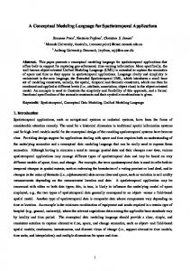
delete(T, ψ, tb, !TBV )@` deletes all rows matching the pattern T and the predicate ψ from table tb in the database located at `, and binds the deleted rows to the table variable TBV . The language has two variants of “selection”: an “external” one that selects data from tables actually existing in databases, identified by their table identifiers, and an “internal” one that selects data from temporary tables bound to table variables. The action sel ext(T, ψ, tb, t, !TBV )@` performs the “external” selection. It picks all rows matching the pattern T as well as satisfying the predicate ψ, from the table identified by tb of the database located at `, and binds the resulting table into the table variable TBV . On the other hand, sel int(T, ψ, TBV , t, !TBV 0 ) performs the “internal” selection, i.e., from the content of the table variable TBV , and binds the resulting table further into the table variable TBV 0 . In sel int(T, ψ, TBV , t, !TBV 0 ), the meanings of T , ψ, and t are the same as those in sel ext(T, ψ, tb, t, !TBV )@`. In both variants, we require that each component of t should be a value or a bound variable of T . The action update(T, ψ, t, tb)@` replaces each row matching T yet satisfying ψ in table tb (at `) with a new row t, while leaving the rest of the rows unchanged. It is required that fv (t) ⊆ bv (T ). The action aggr(T, ψ, tb, f, T 0 )@` applies the aggregation function f on the multiset of all rows meeting T and ψ in table tb (at `) and binds the aggregation result to the pattern T 0 . The action create(I)@` (resp. drop(tb)@`) creates a table identified by I (resp. drops the table identified by tb) in the database at `. An item is a row in a table containing sequences of values, which can be obtained from the evaluation of an expression e. Pattern-matching is used to manage the data inside a table by means of a given template T , which is a sequence of values and variables. Setting the Scene for the Running Example Consider the management of a large-scale chain of department stores, in which the head office can manage the sales of different imaginative brands (e.g., KLD, SH,...) in its individual branches, as shown in Figure 1. We will use underlined symbols for logical and physical localities, as well as allocation environments, to distinguish between their uses in the example and

elsewhere (e.g., in the semantics). Suppose the database of the head office is maintained on machine s0 and the databases of its branches are maintained on machines s1 to sn . The site s0 has the local environment ρ0 = [self 7→ s0 ][`1 7→ s1 ]...[`n 7→ sn ]. We use ρj = [self 7→ sj ] as the local environment for each site sj — this restricts database accesses across different local databases and corresponds to a centralized architecture. City Address Shop Name Brand Logical Locality CPH ABC DEF 2, 1050 Shop1 {KLD, SH, ...} `1 CPH DEF HIJ 13, 2800 Shop2 {KLD, SH, ...} `2 CPH HIJ KLM 26, 1750 Shop3 {KLD, SH, ...} `3 AAL KLM NOP 3, 3570 Shop4 {LAM, IM K, ...} `4 AAL NOP QUW 18, 4500 Shop5 {LAM, IM K, ...} `5 ... ... ... ... ... Fig. 2. The Table Stores

A table with identifier Stores exists in the database of the head office, and records the information of its branches, as shown in Figure 2. The header partially describes the schema I0 of the table, and the subsequent rows, constituting the multiset R0 , contain the information of the different branches. Formally, we have I0 .id = Stores, I0 .sk =< “City” : String, “Address” : String, “Shop name” : String, “Brand” : Set, “Logical Locality” : String >. Each database of a branch has several tables identified by the name of the brand, which record the information of the stock and sales of the corresponding brand. The table of one shoe brand, KLD, in one branch, is shown in Figure 3. The identifier of this table is KLD and the schema is < “Shoe ID” : String, “Shoe name” : String, “Y ear” : String, “Color” : String, “Size” : Int, “In-stock” : Int, “Sales” : Int >. Shoe ID 001 001 001 001 001 002 002 ...

Shoe name HighBoot HighBoot HighBoot HighBoot HighBoot ShortBoot ShortBoot ...

Year Color Size In-stock Sales 2015 red 38 5 2 2015 red 37 8 5 2015 red 36 3 1 2015 black 38 3 2 2015 black 37 5 2 2015 green 38 2 0 2015 brown 37 4 3 ... ... ... ... ...

Fig. 3. The Table KLD in one branch

To sum up, the network of databases and operating processes can be represented by s0 ::ρ0 ((I0 , R0 )|C00 ) || s1 ::ρ1 ((I1 , R1 )|C10 ) || ... || sn ::ρn ((In , Rn )|Cn0 ),

where for j ∈ {1, ..., n}, (Ij , Rj ) describes the local table for the brand KLD inside its database at sj , and for each k ∈ {0, ..., n}, Ck0 stands for the remaining processes and tables at the site sk .

3

Semantics

We devise a structural operational semantics [8] for Klaim-DB, as shown in Table 3 and Table 4. The semantics is defined with the help of a structural congruence — the smallest congruence relation satisfying the rules in Table 2, where the α-equivalence of N and N 0 is denoted by N ≡α N 0 . Table 2. The Structural Congruence N1 ||N2 ≡ N2 ||N1 (N1 ||N2 )||N3 ≡ N1 ||(N2 ||N3 ) N ||nil ≡ N N ≡ N 0 (if N ≡α N 0 )

(νs1 )(νs2 )N ≡ (νs2 )(νs1 )N N1 ||(νs)N2 ≡ (νs)N1 ||N2 (if s 6∈ fn(N1 )) s ::ρ C ≡ s ::ρ C|nil s ::ρ (C1 |C2 ) ≡ s ::ρ C1 || s ::ρ C2

We start by explaining our notation used in the semantic rules. The evaluation function EJ·Kρ evaluates tuples and templates under the allocation environment ρ. The evaluation is performed pointwise on all the components of tuples t and templates T , much in the manner of standard Klaim [2]. We denote by [a/b] the substitution of a for b; in particular, when a and b are tuples of the same length, point-wise substitution is represented. Pattern matching is performed with the help of the predicate match(eT, et) where eT is an evaluated template and et is an evaluated tuple. This match(eT, et) can be defined in a manner much like that of [2]. In more detail, match(eT, et) gives a boolean value indicating whether the pattern matching succeeded. In case it did, the substitution σ = [et/eT ] can be resulted. For example, match((3, !x, !y), (3, 5, 7)) = true and [(3, 5, 7)/(3, !x, !y)] = [5/x, 7/y]. We denote by ψσ the fact that the boolean formula ψ is satisfied after the substitution σ is applied to it. We will use ], ∩ and \ to represent the union, intersection and substraction, of multisets and the detailed definitions are given in Appendix A. The notation I[a 7→ b][...] represents the update of the interface I that maps its attribute a to b; multiple updates are allowed. In addition, we will use I.sk ↓ Tt to represent the projection of the schema I.sk according to the template T (matching the format requirements imposed by I.sk ) and the tuple t. When t only contains constants or the bound variables of T as its components, I.sk ↓ Tt is a new schema that describes only the columns referred to in the variable components of t. Since we have left the schema under-specified, this projection operation is illustrated in Example 1, rather than formally defined. Example 1. Suppose I.sk =< “Shoe ID” : String, “Shoe name” : String, “Y ear” : String, “Color” : String, “Size” : Int, “In-stock” : Int, “Sales” : Int >, which specifies that the table having I as its interface has seven columns: “Shoe ID00 of type String, “Shoe name” of type String, “Year” of type String, “Color” of type String, “Size” of type Int, “In-stock” of type Int, “Sales” of type Int. Suppose in addition that T = (“001”, “HighBoot”, !x, !y, !z, !w, !p) and t = (y, z, p). Then I.sk ↓ Tt =< “Color” : String, “Size” : Int, “Sales” : Int >. t u

Table 3. The Semantics for Actions

(INS)

(INS TB)

ρ1 (l) = s2 I.id = tb t |= I.sk R0 = R ] {EJtKρ1 } s1 ::ρ1 insert(t, tb)@`.P || s2 ::ρ2 (I, R) → s1 ::ρ1 P || s2 ::ρ2 (I, R0 ) ρ1 (l) = s2 I.id = tb I 0 .sk = I.sk R00 = R ] R0

s1 ::ρ1 insert tb((I 0 , R0 ), tb)@`.P || s2 ::ρ2 (I, R) → s1 ::ρ1 P || s2 ::ρ2 (I, R00 ) R0 = {t | t ∈ R ∧ ¬(match(EJT Kρ1 , t) ∧ ψ[t/EJT Kρ1 ])} R00 = {t | t ∈ R ∧ match(EJT Kρ1 , t) ∧ ψ[t/EJT Kρ1 ]} ρ1 (l) = s2 I.id = tb σ 0 = [(I, R00 )/TBV ]

(DEL)

s1 ::ρ1 delete(T, ψ, tb, !TBV )@`.P || s2 ::ρ2 (I, R) → s1 ::ρ1 P σ 0 || s2 ::ρ2 (I, R0 )

(SEL EXT)

ρ1 (l) = s2 I.id = tb I 0 = I[id 7→ ⊥][sk 7→ I.sk ↓Tt ] σ 0 = [(I 0 , R0 )/TBV ] R0 = {EJtσKρ1 | ∃t0 : t0 ∈ R ∧ match(EJT Kρ1 , t0 ) ∧ σ = [t0 /EJT Kρ1 ] ∧ ψσ}

s1 ::ρ1 sel ext(T, ψ, tb, t, !TBV )@`.P || s2 ::ρ2 (I, R) → s1 ::ρ1 P σ 0 || s2 ::ρ2 (I, R) I 0 = I[id 7→ ⊥][sk 7→ I.sk ↓Tt ] σ 0 = [(I 0 , R0 )/TBV ] 0 0 0 0 (SEL INT) R = {EJtσKρ1 | ∃t : t ∈ R ∧ match(EJT Kρ1 , t ) ∧ σ = [t /EJT Kρ1 ] ∧ ψσ} s1 ::ρ1 sel int(T, ψ, (I, R), t, !TBV ).P → s1 ::ρ1 P σ 0 0

ρ1 (l) = s2 I.id = tb R10 = {t0 | t0 ∈ R ∧ ¬(∃σ : match(EJT Kρ1 , t0 ) ∧ σ = [t0 /EJT Kρ1 ] ∧ ψσ ∧ EJtσKρ1 |= I.sk)} (UPD) R0 = {EJtσK | ∃t0 : t0 ∈ R ∧ match(EJT K , t0 ) ∧ σ = [t0 /EJT K ] ∧ ψσ ∧ EJtσK |= I.sk} ρ1 ρ1 ρ1 ρ1 2 s1 ::ρ1 update(T, ψ, t, tb)@`.P || s2 ::ρ2 (I, R) → s1 ::ρ1 P ||s2 ::ρ2 (I, R10 ] R20 )

(AGGR)

t0 = f ({t | ∃σ 0 : t ∈ R ∧ match(EJT Kρ1 , t) ∧ σ 0 = [t/EJT Kρ1 ] ∧ ψσ 0 ) ρ(l) = s2 I.id = tb match(EJT 0 Kρ1 , t0 ) s1 ::ρ1 aggr(T, ψ, tb, f, T 0 )@`.P || s2 ::ρ2 (I, R) → s1 ::ρ1 P [t0 /EJT 0 Kρ1 ] || s2 ::ρ2 (I, R)

(CREATE)

(DROP)

ρ1 (l) = s2 s1 ::ρ1 create(I)@`.P ||s2 ::ρ2 nil → s1 ::ρ1 P ||s2 ::ρ2 (I, ∅) ρ1 (l) = s2 I.id = tb

s1 ::ρ1 drop(tb)@`.P ||s2 ::ρ2 (I, R) → s1 ::ρ1 P ||s2 ::ρ2 nil

We proceed with a detailed explanation of the semantic rules in Table 3 that account for the execution of Klaim-DB actions and the ones in Table 4 that mainly describe the execution of the control flow constructs. In the explanation, we will avoid reiterating that each table resides in a database located at some `, but directly state “table ... located at `”. 3.1

Semantics for Actions

Insertion and Deletion The rule (INS) of Table 3 says that to insert a row t into a table tb at s2 , the logical locality ` needs to be evaluated to s2 under the local environment ρ1 , the table identifier tb must agree with that of a destination table (I, R) already existing at s2 , and the tuple t needs to satisfy the requirements imposed by the schema I.sk. If these conditions are met, then the evaluated tuple is added into the data set R. Example 2 (Adding new Shoes). The local action at s1 that inserts an entry for KLD high boots of a new color, white, sized “37”, produced in 2015, with 6 in stock, is insert(T0 , KLD)@self , where T0 = (“001”, “HighBoot”, “2015”, “white”, “37”, 6, 0). By (INS), we have s1 ::ρ1 insert(T0 , KLD)@self .nil || s1 ::ρ1 (I1 , R1 ) → s1 ::ρ1 nil || s1 ::ρ1 (I1 , R10 ),

where R10 = R1 ] {T0 }, since ρ1 (self ) = s1 , KLD = I1 .id and T0 |= I1 .sk .

t u

Deletion operations are performed according to the rule (DEL). A deletion can be performed if the logical locality ` refers to the physical locality s2 under the local environment ρ1 , and the specified table identifier tb agrees with that of the table (I, R) targeted. The rows that do not match the pattern T or do not satisfy the condition ψ will constitute the resulting data set of the target. Example 3 (Deleting Existing Shoes). The local action at `1 , deleting all entries for white KLD high boots sized “37” produced in 2015, from the resulting table of Example 2, is delete(T0 , true, KLD)@self , where T0 = (“001”, “HighBoot”, “2015”, “W hite”, “37”, !x, !y). We have the transition: s1 ::ρ1 delete(T0 , true, KLD)@self .nil || s1 ::ρ1 (I1 , R10 ) → s1 ::ρ1 nil || s1 ::ρ1 (I1 , R1 ).

This reflects that the original table is recovered after the deletion.

t u

Selection, Update and Aggregation The rule (SEL EXT) describes the way the “external” selection operations are performed. It needs to be guaranteed that the logical locality ` is evaluated to s2 (under the local environment ρ1 ), and the identifier tb is identical to that of the table (I, R) existing at s2 . If the conditions are met, all the rows that match the pattern T and satisfy the predicate ψ, will be put into the result data set R0 . The schema of the resulting table is also updated according to the pattern T and the tuple t. The resulting table (I 0 , R0 ) is substituted into each occurrence of the table variable TBV used in the continuation P .

Example 4 (Selection of Shoes in a Certain Color). The Klaim-DB action performed from the head office, selecting the color, size, and sales of the types of high boots that are not red, at the local database at s1 , is sel ext((“001”, “HighBoot”, !x, !y, !z, !w, !p), y 6= “red”, KLD, (y, z, p), !TBV )@`1 .

According to the rule (SEL EXT), we have the transition: s0 ::ρ0 sel ext((“001”, “HighBoot”, !x, !y, !z, !w, !p), y 6= “red”, KLD, (y, z, p), !TBV )@`1 .nil || s1 ::ρ1 (I1 , R1 ) → s0 ::ρ0 nil || s1 ::ρ1 (I1 , R1 ).

The conditions ρ0 (`1 ) = s1 and KLD = I.id in the premises of the rule are satisfied. The I 0 in (SEL EXT) is such that I 0 .id = ⊥, I 0 .sk =< “Color” : String, “Size” : Int, “Sales” : Int >, and I 0 agrees with I on the other attributes. The table variable TBV is replaced by (I 0 , R0 ), for some R0 = {(“black”, “38”, “2”), (“black”, “37”, “2”)}. t u “Internal” selections are performed according to the rule (SEL INT). No constraints concerning localities/identifiers are needed. All the rows that match the pattern T and satisfy the predicate ψ are selected into the resulting data set R0 . The schema of the result table is produced by using the projection operation introduced in the beginning of this section. All occurrences of the table variable TBV in the continuation P will be replaced by the resulting table (I 0 , R0 ) before continuing with further transitions. We use ⊥ for I 0 .id to indicate that (I 0 , R0 ) is a “temporary” table that can be thought of as existing in the query engine, rather than in the database. The updates of data stored in tables are executed according to the rule (UPD). Again, it is checked that the specified logical locality of the table (I, R) to be updated corresponds to the site where the table actually resides, and that the specified table identifier matches the actual one. An update goes through all the elements t0 of R. This t0 is updated only if it matches the template T , resulting in the substitution σ that makes the predicate ψ satisfied, and tσ is evaluated to a tuple that satisfies the schema I.sk. The evaluation result of tσ will then replace t0 in the original table, which is captured by R20 . If at least one of the above mentioned conditions is not met, then t0 will be left intact (described by R10 ). Example 5 (Update of Shoes Information). Suppose two more red KLD high boots sized 37 are sold. The following local action informs the database at s1 of this. update( (“001”, “HighBoot”, “2015”, “red”, “37”, !x, !y), true, (“001”, “HighBoot”, “2015”, “red”, “37”, x − 2, y + 2), KLD)@self .

We have the transition: s1 ::ρ1 update((“001”, “HighBoot”, “2015”, “red”, “37”, !x, !y), true, (“001”, “HighBoot”, “2015”, “red”, “37”, x − 2, y + 2), KLD)@self .nil || s1 ::ρ1 (I, R) → s1 ::ρ1 nil || s1 ::ρ1 (I, R10 ] R20 ).

The multiset R10 consists of all the entries that are intact — shoes that are not t u red high boots sized 37, while R20 contains all the updated items.

The rule (AGGR) describes the way aggregation operations are performed. The matching of localities and table identifiers is still required. The aggregation function f is applied to the multiset of all tuples matching the template T , as well as satisfying the predicate ψ. The aggregation result t0 obtained by the application of f is bound to the specified template T 0 only if the evaluation of T 0 matches t0 . In that case the substitution reflecting the binding is applied to the continuation P and the aggregation is completed. Example 6 (Aggregation of Sales Figures). The local aggregation returning the total sales of the shoes with ID “001”, can be modelled by the Klaim-DB action aggr(T0 , true, KLD, sum 7 , (!res))@self , where T0 = (“001”, !x, !y, !z, !w, !q, !o), and sum 7 = λR.(sum({v7 |(v1 , ..., v7 ) ∈ R})), i.e., sum 7 is a function from multisets R to unary tuples containing the summation results of the 7-th components of the tuples in R. It is not difficult to derive: s1 ::ρ1 aggr(T0 , true, KLD, sum 7 , (!res))@`1 .nil || s1 ::ρ1 (I, R) → s1 ::ρ1 nil || s1 ::ρ1 (I, R).

The variable !res is then bound to the integer value 12 (2 + 5 + 1 + 2 + 2).

t u

Example 7 (Selection using Aggregation Results). Consider the query from s0 that selects all the colors, sizes and sales of the types of high boots produced in the year 2015, whose ID is “001” and whose sales figures are above average. This query can be modelled as a sequence of actions at s0 , as follows. s0 ::ρ0 aggr(T0 , true, KLD, avg 7 , !res)@`1 .sel ext(T0 , w ≥ res, KLD, (x, y, w), !TBV )@`1 .nil || s1 ::ρ1 (I1 , R1 ),

where T0 = (“00100 , “HighBoot”, “2015”, !x, !y, !z, !w) and 1 ,...,v7 )∈R}) avg 7 = λR.( sum({v7 |(v|R| ) is a function from multisets R to unary tuples containing the average value of the 7-th components of the tuples in R. t u Adding and Dropping Tables To create a new table, the rule (CREATE) ensures that the physical site s2 corresponding to the logical locality ` mentioned in the action create(I)@` does exist. Then a table with the interface I and an empty data set is created at the specified site. It remains an issue to ascertain that there are no existing tables having the same identifier I.id at the target site. This is achieved with the help of the rule (PAR) in Table 4. To drop an existing table, the rule (DROP) checks that a table with the specified identifier tb does exist at the specified site ρ1 (l) = s2 . Then the table is dropped by replacement of it with nil. 3.2

Semantics for Processes and Networks

ff Directing our attention to Table 4, the rules (FORtt s ) and (FORs ) specify when and how a loop is to be executed one more time, and has finished, respectively.

Table 4. The Semantics for Processes and Nets (Continued)

(FORtt s )

(FORtt p)

(FORffs )

(SEQtt )

t0 ∈ R match(EJT Kρ , t0 )

s ::ρ foreachs T in R : P → s ::ρ P [t0 /EJT Kρ ]; foreachs T in R \ {t0 } : P t0 ∈ R match(EJT Kρ , t0 )

s ::ρ foreachp T in R : P → s ::ρ P [t0 /EJT Kρ ] | foreachp T in R \ {t0 } : P

¬(∃t0 ∈ R : match(EJT Kρ , t0 ))

s ::ρ foreachs T in R : P → s ::ρ nil s ::ρ P1 || N → s ::ρ P10 || N 0 s ::ρ P1 ; P2 || N → s ::ρ P10 ; P2 || N 0

(FORffp )

¬(∃t0 ∈ R : match(EJT Kρ , t0 ))

s ::ρ foreachp T in R : P → s ::ρ nil

(SEQff )

s ::ρ P1 || N → s ::ρ nil || N 0 s ::ρ P1 ; P2 || N → s ::ρ P2 || N 0

(CALL) s ::ρ A(t˜) → s ::ρ P [˜ v /˜ x] if A(˜ x) , P ∧ EJt˜Kρ = v˜ (PAR)

(RES)

N1 → N10 N1 ||N2 → N10 ||N2

N → N0 (νs)N → (νs)N 0

if Lid (N10 ) ∩ Lid (N2 ) = ∅

(EQUIV)

N1 ≡ N2 N2 → N3 N3 ≡ N4 N1 → N4

The rule (FORtt s ) says that if there are still more tuples (e.g., t0 ) in the multiset R matching the pattern specified by the template T , then we first execute one round of the loop with the instantiation of variables in T by corresponding values in t0 , and then continue with the remaining rounds of the loop by removing t0 from R. The rule (FORffs ) says that if there are no more tuples in R matching T , ff then the loop is completed. The rules (FORtt p ) and (FORp ) can be understood similarly. The rules (SEQtt ) and (SEQff ) describe the transitions that can be performed by sequential compositions P1 ; P2 . In particular, the rule (SEQtt ) accounts for the case where P1 cannot finish after one more step; whereas the rule (SEQff ) accounts for the opposite case. We require that no variable bound in P1 is used in P2 , thereby avoiding the need for recording the substitutions resulting from the next step of P1 , that need to be applied on P2 . The rule (PAR) says that if a net N1 can make a transition, then its parallel composition with another net N2 can also make a transition, as long as no clashes of table identifiers local to each site in N1 ||N2 are introduced. It makes use of the function Lid (...) that gives the multiset of pairs of physical localities and table identifiers in networks and components. This function is overloaded on networks

and components, and is defined inductively as follows. Lid (nil) = ∅ Lid (s, P ) = ∅ Lid (N1 ||N2 ) = Lid (N1 ) ] Lid (N2 ) Lid (s, (I, R)) = {(s, I.id)} Lid ((νs)N ) = Lid (N ) Lid (s, C1 |C2 ) = Lid (s, C1 ) ] Lid (s, C2 ) Lid (s ::ρ C) = Lid (s, C)

The rules (CALL), (RES) and (EQUIV) are self-explanatory. It is a property of our semantics that no local repetition of table identifiers can be caused by a transition (including the creation of a new table). Define no rep(A) = (A = set(A)), which expresses that there is no repetition in the multiset A, thus A coincides with its underlying set. This property is formalized in Lemma 1 whose proof is straightforward by induction on the derivation of the transition. Lemma 1. For all nets N and N 0 , if no rep(Lid (N )) and N → N 0 , then it holds that no rep(Lid (N 0 )). Thus, imposing “non-existence of local repetition of table identifiers” as an integrity condition for the initial network will guarantee the satisfaction of this condition in all possible derivatives of the network. Example 8 (Transition of Networks). Continuing with Example 2, we illustrate how our semantics help establish global transitions. Suppose there is no other table at s1 with the identifier KLD. By (PAR), and the structural congruence, we have s0 ::ρ0 (I0 , R0 )|C00 || s1 ::ρ1 (I1 , R1 )|insert(t1 , KLD)@self .nil|C100 || ... || sn ::ρn (In , Rn )|Cn0 → s0 ::ρ0 (I0 , R0 )|C00 || s1 ::ρ1 (I1 , R10 )|C100 || ... || sn ::ρn (In , Rn )|Cn0 ,

where t1 = (“001”, “HighBoot”, “2015”, “white”, “37”, “6”, “0”).

4

t u

Case Study

Continuing with our running example, we illustrate the modelling of data aggregation over multiple databases local to different branches of the department store chain in Klaim-DB. In more detail, a manager of the head office wants statistics on the total sales of KLD high boots from the year 2015, in each branch operating in Copenhagen. We will think of a procedure stat at the site s0 of the head office, carrying out the aggregation needed. Thus the net for the database systems of the department store chain, as considered in Section 2, specializes to the following, where C000 is the remaining tables and processes at s0 apart from Stores and stat. s0 ::ρ0 (stat|(I, R)|C000 ) || s1 ::ρ1 ((I1 , R1 )|C10 ) || ... || sn ::ρn ((In , Rn )|Cn0 )

A detailed specification of the procedure stat is then given in Figure 4. First of all, a result table with the interface Ires is created, where Ires .id = result and I.sk =< “Brand” : String, “City” : String, “Shop name” : String,

stat , create(Ires )@self . sel ext((!x, !y, !z, !w, !p), KLD ∈ w ∧ x = “CP H”, Stores, (z, p), !TBV )@self . foreachp (!q, !u) in TBV .R : aggr((“001”, “HighBoot”, “2015”, !x, !y, !z, !w), true, KLD, sum 7 , (!res))@u. insert((q, “HighBoot”, res), result)@self ; ... drop(result)@self Fig. 4. The Procedure for Distributed Data Aggregation

“Sales” : Int >. Then all the logical localities of the local databases used by the branches in Copenhagen that actually sell KLD shoes are selected, together with the shop names of such branches. This result set is then processed by a parallel loop. The number of KLD high boots from 2015 that are sold is counted at each of these localities (branches), and is inserted into the resulting table together with the corresponding shop name and the information “High Boot” describing the shoe type concerned. The resulting table, displayed in Figure 5, can still be queried/manipulated before being dropped. In the end of this case study, we Shop name Shoe name Sales would like to remark that the use of the parallel loop in carrying out Shop1 HighBoot 12 all the individual remote aggregations Shop2 HighBoot 53 has made the overall query more efShop3 HighBoot 3 ficient. Hence some performance is... ... ... sues can be captured by modelling in Fig. 5. The Table result Klaim-DB.

5

Extension and Discussion

Joining Tables Our modelling language can be extended to support querying from the “join” of tables. For this extension, we make use of under-specified join expressions je, that can have table identifiers or table variables as parameters. The syntax of the new selection actions is shown below. a ::= ... | sel ext(T, ψ, je(tb 1 , ..., tb n ), t, !TBV )@`1 , ..., `n | sel int(T, ψ, je(TBV 1 , ..., TBV n ), t, !TBV 0 ) | ...

For an external selection, we allow to use a list `1 , ..., `n of localities (abbreviated as `), to join tables located in multiple databases. In more detail, for i ∈ {1, ..., n}, tb i is supposed to be the identifier of a table located at `i . We use JjeKR and JjeKI to represent the interpretation of je in terms of how the datasets and the schemas of the joined tables should be combined. As an example, a plain list of table identifiers or tables (substitution of table variables) corresponds to taking the concatenation of all the schemas and selecting from the cartesian product of all the data sets. JjeKI (I1 , ..., In ) =

M

Ij .sk

j∈{1,...,n}

JjeKR (R1 , ..., Rn ) = R1 × ... × Rn

Table 5. The Semantic Rules for Selection from Joins n = |tb| = |`| ∧ ∀j ∈ {1, ..., n} : ρ0 (lj ) = sj ∧ tb j = Ij .id σ 0 = [(I 0 , R0 )/TBV ] I 0 = [id 7→ ⊥][sk 7→ (JjeKI (I)) ↓Tt ] 0 0 R 0 0 0 (SELJ EXT) R = {EJtσKρ1 | ∃t : t ∈ JjeK (R) ∧ match(EJT Kρ1 , t ) ∧ σ = (t /EJT Kρ1 ) ∧ ψσ} s0 ::ρ0 sel ext(T, ψ, je(tb), t, !TBV )@`.P || s1 ::ρ1 (I1 , R1 ) || ... || sn ::ρn (In , Rn ) → s0 ::ρ0 P σ 0 || s1 ::ρ1 (I1 , R1 ) || ... || sn ::ρn (In , Rn ) I 0 = [id 7→ ⊥][sk 7→ (JjeKI (I)) ↓Tt ] σ 0 = [(I 0 , R0 )/TBV ] 0 0 R 0 0 0 (SELJ INT) R = {EJtσKρ1 | ∃t : t ∈ JjeK (R) ∧ match(EJT Kρ1 , t ) ∧ σ = (t /EJT Kρ1 ) ∧ ψσ} s1 ::ρ1 sel int(T, ψ, je((I, R)), t, !TBV ).P → s1 ::ρ1 P σ 0

The pattern matching against the template T and the satisfaction of the predicate ψ will be examined on tuples from JjeKR (R1 , ..., Rn ), and the predicate ψ can now impose constraints on the fields from different tables. The adaption needed for the semantics is fairly straightforward. The semantic rules (SELJ EXT) and (SELJ INT) that describe selection operations from joined tables are presented in Table 5. In the rule (SELJ EXT), although it is stipulated that the j-th table identifier specified in the list tb must be identical to the j-th table (Ij , Rj ) listed as parallel components, no undesired stuck configurations are caused because of the structrual congruence. This extension paves the way for the general ability to operate on multiple databases by a single action, which is in line with the design philosophy of multidatabase systems (e.g., [5]). Discussion We could have required whole tables to be received into local variables by using the standard Klaim actions out(t)@` and in(t)@`, and made the selection and aggregation operations work only on table variables. In this way we could have gotten rid of “external selection”. However, “external selection” on remote localities can potentially reduce the communication cost considerably, since only one tuple (for aggregation) or a part of a table (for selection) need to be returned. For selection the reduction is particularly meaningful when the resulting data set is small. Concerning the result of selection operations, an alternative that we have not adopted is the direct placement of the result in a separate table. This table is either created automatically by the selection operation itself, with an identifier specified in the selection action, or a designated “result table” at each site. However, a problem is that the removal of the automatically created tables will need to be taken care of by the system designer making the specification, using drop(I)@` actions. And similar problems arise with the maintenance of the designated “result table” local to each site (e.g., the alteration of its schema, the cleaning of old results, etc.). To abstain from these low-level considerations, table variables are introduced and binding is used for the selection results.

The interoperability between database systems and ordinary applications can also be realized by bringing back the primitive Klaim actions (out(t)@`, in(T )@`, and eval(P )@`) and allowing the co-existence of tables and plain tuples at different localities. Via the re-introduction of the eval action, we would also be able to send out mobile processes to perform complex data processing on-site.

6

Conclusion

We have proposed Klaim-DB — a modelling language that borrows insights from both the coordination language Klaim and database query languages like SQL, to support the high-level modelling and reasoning of distributed database applications. The semantics is illustrated with a running example on the query and management of the databases used by a department store chain. Data aggregation across the geographically scattered databases at the individual stores, as performed by a coordinator, is then modelled in the language. In the model, the local aggregations at the store-owned databases are performed in parallel with each other, benefiting the performance. Our use of templates in the query actions of Klaim-DB is in line with the spirit of the QBE language (Query by Example [12]). The choice of using multiset operations for the semantics of these actions, on the other hand, has the flavor of the Domain Relational Calculus underlying QBE. The work presented in [9] discusses typical coordination issues in distributed databases in Linda, from an informal, architectural viewpoint. This work is marginally related to ours. The specification and enforcement of security policies is an important concern in distributed database systems. A simple example is: when inserting data into a remote table, it is important to know whether the current site trusts the remote site with respect to confidentiality, and whether the remote site trusts the current site with respect to integrity. Recently, [3] and [7] address privacy and information flow issues in database applications. Another work, [10], provides an information flow analysis for locality-based security policies in Klaim. By elaborating on the language design, we provide in this paper a solid ground for any future work aiming to support security policies and mechanisms. Another interesting line of future work is the specification of transactions (e.g., [6]). This is needed for the modelling of finer-grained coordination between database accesses. Acknowledgment. We would like to thank the anonymous reviewers for their valuable feedback. Xi Wu is partly supported by the IDEA4CPS project, ECNU Project of Funding Overseas Short-term Studies, Domestic Academic Visit and NSFC Project (No.61361136002 and No.61321064). Ximeng Li is partly funded by SESAMO, a European Artemis project.

References 1. Jean-Raymond Abrial. Formal methods: Theory becoming practice. J. UCS, 13(5):619–628, 2007.

2. Rocco De Nicola, Gian Luigi Ferrari, and Rosario Pugliese. KLAIM: A kernel language for agents interaction and mobility. IEEE Trans. Software Eng., 1998. 3. Cynthia Dwork. Differential privacy. In Encyclopedia of Cryptography and Security, 2nd Ed., pages 338–340. 2011. 4. C. A. R. Hoare. Communicating Sequential Processes. Prentice-Hall, 1985. 5. E. Kuhn and T. Ludwig. Vip-mdbs: A logic multidatabase system. In Proceedings of the First International Symposium on Databases in Parallel and Distributed Systems, DPDS ’88, pages 190–201. IEEE Computer Society Press. 6. Eva K¨ uhn, Ahmed K. Elmagarmid, Yungho Leu, and Noureddine Boudriga. A parallel logic language for transaction specification in multidatabase systems. Journal of Systems Integration, 5(3):219–252, 1995. 7. Lu´ısa Louren¸co and Lu´ıs Caires. Information flow analysis for valued-indexed data security compartments. In Trustworthy Global Computing - 8th International Symposium, TGC 2013, pages 180–198, 2013. 8. Gordon D. Plotkin. A structural approach to operational semantics. J. Log. Algebr. Program., 60-61:17–139, 2004. 9. Madhan M Thirukonda and Ronaldo Menezes. On the use of linda as a framework for distributed database systems. 2002. 10. Terkel K. Tolstrup, Flemming Nielson, and Ren´e Rydhof Hansen. Locality-based security policies. In Formal Aspects in Security and Trust, Fourth International Workshop, FAST 2006, pages 185–201, 2006. 11. Jim Woodcock, Peter Gorm Larsen, Juan Bicarregui, and John S. Fitzgerald. Formal methods: Practice and experience. ACM Comput. Surv., 41(4), 2009. 12. Mosh´e M. Zloof. Query by example. In Proceedings of the May 19-22, 1975, National Computer Conference and Exposition, AFIPS ’75, pages 431–438, New York, NY, USA, 1975. ACM.

A

Multiset Notation

We use ], ∩ and \ to represent the union, intersection and substraction, respectively, of multisets. For a multiset S, and an element s, the application M (S, s) of the multiplicity function M gives the number of repetitions of s in S. Note that for s 6∈ S, M (S, s) = 0. Then our notions of union, intersection and subtraction are such that M (S1 ] S2 , s) = M (S1 , s) + M (S2 , s) M (S1 ∩ S2 , s) = min(M (S1 , s), M (S2 , s)) M (S1 \ S2 , s) = abs(M (S1 , s) − M (S2 , s)) Here abs(v) gives the absolute value of the integer v.