A Rule-Driven Dynamic Programming Decoder for Statistical MT

A Rule-Driven Dynamic Programming Decoder for Statistical MT

Christoph Tillmann IBM T.J. Watson Research Center Yorktown Heights, N.Y. 10598 [email protected]

Abstract The paper presents an extension of a dynamic programming (DP) decoder for phrase-based SMT (Koehn, 2004; Och and Ney, 2004) that tightly integrates POS-based re-order rules (Crego and Marino, 2006) into a left-to-right beam-search algorithm, rather than handling them in a pre-processing or re-order graph generation step. The novel decoding algorithm can handle tens of thousands of rules efficiently. An improvement over a standard phrase-based decoder is shown on an ArabicEnglish translation task with respect to translation accuracy and speed for large re-order window sizes.

1

Introduction

The paper presents an extension of a dynamic programming (DP) decoder for phrase-based SMT (Koehn, 2004; Och and Ney, 2004) where POSbased re-order rules (Crego and Marino, 2006) are tightly integrated into a left-to-right run over the input sentence. In the literature, re-order rules are applied to the source and/or target sentence as a pre-processing step (Xia and McCord, 2004; Collins et al., 2005; Wang et al., 2007) where the rules can be applied on both training and test data. Another way of incorporating re-order rules is via extended monotone search graphs (Crego and Marino, 2006) or lattices (Zhang et al., 2007; Paulik et al., 2007). This paper presents a way of handling POS-based re-order rules as an edge generation process: the POS-based re-order rules are tightly integrated into a left to right beam search decoder in a way that

29 000 rules which may overlap in an arbitrary way (but not recursively) are handled efficiently. Example rules which are used to control the novel DP-based decoder are shown in Table 1, where each POS sequence is associated with possibly several permutations π. In order to apply the rules, the input sentences are POS-tagged. If a POS sequence of a rule matches some identical POS sequence in the input sentence the corresponding words are re-ordered according to π. The contributions of this paper are as follows: 1) The novel DP decoder can handle tens of thousands of POS-based rules efficiently rather than a few dozen rules as is typically reported in the SMT literature by tightly integrating them into a beam search algorithm. As a result phrase re-ordering with a large distortion window can be carried out efficiently and reliably. 2) The current rule-driven decoder is a first step towards including more complex rules, i.e. syntax-based rules as in (Wang et al., 2007) or chunk rules as in (Zhang et al., 2007) using a decoding algorithm that is conceptually similar to an Earley-style parser (Earley, 1970). More generally, ’rule-driven’ decoding is tightly linked to standard phrase-based decoding. In future, the edge generation technique presented in this paper might be extended to handle hierarchical rules (Chiang, 2007) in a simple left-to-right beam search decoder. In the next section, we briefly summarize the baseline decoder. Section 3 shows the novel ruledriven DP decoder. Section 4 shows how the current decoder is related to both DP-based decoding algorithms in speech recognition and parsing. Finally,

37 Proceedings of the Second ACL Workshop on Syntax and Structure in Statistical Translation (SSST-2), pages 37–45, c ACL-08: HLT, Columbus, Ohio, USA, June 2008. 2008 Association for Computational Linguistics

Table 1: A list of 28 878 reorder rules sorted according to the rule occurrence count N (r) is used in this paper. For each POS sequence the corresponding permutation π is shown. Rule ID is the ordinal number of a rule in the sorted list. The maximum rule length that can be handled efficiently is surprisingly long: about 20 words. Rule ID r POS sequence π N (r) 1 DET NOUN DET ADJ → 2301 4 421 2 DET NOUN NSUFF-FEM-SG DET ADJ NSUFF-FEM-SG → 345012 2 257 .. .. .. . . . 3 000 NOUN CASE-INDEF-ACC ADJ NSUFF-FEM-SG CONJ ADJ NSUFF-FEM-SG → 2345601 6 .. .. .. . . . 28 878 PREP DET NOUN DET ADJ PREP NOUN-PROP ADJ → 0127834 NSUFF-MASC-SG-ACC-INDEF CONJ IV3MS IV IVSUFF-DO:3FS 9 10 11 12 5 6 2

Section 5 shows experimental results.

2

Baseline DP Decoder

The translation model used in this paper is a phrasebased model (Koehn et al., 2003), where the translation units are so-called blocks: a block b is a pair consisting of a source phrase s and a target phrase t which are translations of each other. The expression block is used here to emphasize that pairs of phrases (especially longer phrases) tend to form closely linked units in such a way that the translation process can be formalized as a block segmentation process (Nagata et al., 2006; Tillmann and Zhang, 2007). Here, the input sentence is segmented from left to right while simultaneously generating the target sentence, one block at a time. In practice, phrase-based or block-based translation models which largely monotone decoding algorithms obtain close to state-of-the-art performance by using skip and window-based restrictions to reduce the search space (Berger et al., 1996). During decoding, we maximize the score sw (bn1 ) of a phrase-pair sequence bn1 = (si , ti )n1 : sw (bn1 ) =

n X

wT · f (bi , bi−1 ),

(1)

i=1

where bi is a block, bi−1 is its predecessor block, and f (bi , bi−1 ) is a 8-dimensional feature vector where the features are derived from some probabilistic models: language model, translation model, and distortion model probabilities. n is the number of blocks in the translation and the weight vector w is trained in a way as to maximize the decoder BLEU score on some training data using an on-line algorithm (Tillmann and Zhang, 2008). The decoder that 38

carries out the optimization in Eq. 1 is similar to a standard phrase-based decoder (Koehn, 2004; Och and Ney, 2004), where states are tuples of the following type: [ C ; [i, j] ], (2) where C is the so-called coverage vector that keeps track of the already processed source position, [i, j] is the source interval covered by the last source phrase match. In comparison, (Koehn, 2004) uses only the position of the final word of the last source phrase translated. Since we are using the distortion model in (Al-Onaizan and Papineni, 2006) the entire last source phrase interval needs to be stored. Hypothesis score and language model history are omitted for brevity reasons. The states are stored in lists or stacks and DP recombination is used to reduce the size of the search space while extending states. The algorithm described in this paper uses an intermediate data structure called an edge that represents a source phrase together with a target phrase that is one of its possible translation. Formally, we define: [ [i, j] , tN (3) 1 ], where tN 1 is the target phrase linked to the source phrase si , · · · , sj . The edges are stored in a so-called chart. For each input interval that is matched by some source phrase in the block set, a list of possible target phrase translations is stored in the chart. Here, simple edges as in Eq. 3 are used to generate so-called rule edges that are defined later in the paper. A similar data structure corresponding to an edge is called translation option in (Koehn, 2004). While the edge generation potentially slows down the overall decoding process, for the baseline de-

e=2

e=1

e=5

a

a

0

1

e=2

e=1

a

e=1, r=1 p=END ORIG=[0,1]

e=3, r=2

e=1, r=2

p=BEG ORIG=[1,3]

p=END ORIG=[0,1]

e=4, r=3

e=3, r=3

p=INTER ORIG=[3,4]

p=END ORIG=[1,2]

p

4

Additional ’Rule’ Edge Copies

e=1, r=3

a

1

a

2

a

3

a

1

0

1

2 0

0

3 4 1 2

1

p 0

p

’Extended’ Chart

4

p

p

’Original’ Chart

’Simple’ Edges’

p=BEGIN ORIG=[0,1]

0

a

e=4

p=BEG ORIG=[1,2]

0

3.

3

e=5

e=2, r=1

a

2.

a

2

e=3

1.

’Simple’ ’Edges’

e=4

e=3

p 1

p 0

2

p

p 1

2

p 3

4

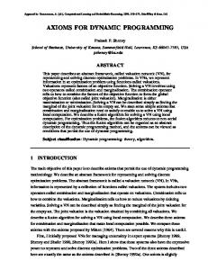
Figure 1: Addition of rule edges to a chart containing 5 simple edges (some rule edges are not shown). The simple edges remain in the chart after the rule edges have been added: they are used to carry out monotone translations.

coder generating all the simple edges takes less than 0.3 % of the overall decoding time.

3

DP-Search with Rules

This section explains the handling of the re-order rules as an edge generation process. Assuming a monotone translation, for the baseline DP decoder (Koehn, 2004) each edge ending at position j can be continued by any edge starting at position j + 1, i.e. the simple edges are fully connected with respect to their start and ending positions. For the rule-driven decoder, all the re-ordering is handled by generating additional edges which are ’copies’ of the simple edges in each rule context in which they occur. Here, a rule edge copy ending at position j is not fully connected with all other edges starting at position j + 1. Once a rule edge copy for a particular rule id r has been processed that edge can be continued only by an edge copy for the same rule until the end of the rule has been reached. To formalize the approach, the search state definition in Eq. 2 is 39

modified as follows: [ s ; [i, j] , r , sr , e ∈ {false, true} ]

(4)

Here, the coverage vector C is replaced by a single number s: a monotone search is carried out and all the source positions up to position s (including s) are covered. [i, j] is the coverage interval for the last source phrase translated (the same as in Eq. 2). r is the rule identifier, i.e. a rule position in the list in Table 1. sr is the starting position for the rule match of rule r in the input sentence, and e is a flag that indicates whether the hypothesis h has covered the entire span of rule r yet. The search starts with the following initial state: [ −1 ; [−1, −1] , −1 , −1 , e = true ] ,

(5)

where the starting positions s, sr , and the coverage interval [i, j] are all initialized with −1, a virtual source position to the left of the uncovered source input. Throughout the search, a rule id of −1 indicates that no rule is currently applied for that hypothesis, i.e. a contiguous source interval to the left of s is covered.

States are extended by finding matching edges and the generation of these edges is illustrated in Fig. 1 for the use of 3 overlapping rules on a source segment of 5 words a0 , · · · , a4 1 . Edges are shown as rectangles where the number on the left inside the box corresponds to the enumeration of the simple edges. In the top half of the picture the simple edges which correspond to 5 phrase-to-phrase translations are shown. In the bottom half all the edges after the rule edge extension are shown (including simple and rule edges). A rule edge contains additional components: the rule id r, a relative edge position p (explained below), and the original source interval of a rule edge before it has been re-ordered. A rule edge is generated from a simple edge via a re-order rule application: the newly generated edges are added into the chart as shown in the lower half of Figure 1. Here, rule 1 and 2 generate two new edges and rule 3 generates three new edges that are added into the chart at their new re-ordered positions, e.g. copies of edge 1 are added for the rule id r = 1 at start position 2, for rule r = 2 at start position 3, and for rule r = 3 at start position 0. Even if an edge copy is added at the same position as the original edge a new copy is needed. The three rules correspond to matching POS sequences, i.e. the Arabic input sentence has been POS tagged and a POS pj has been assigned to each Arabic word aj . The same POS sequence might generate several different permutations which is not shown here. More formally, the edge generation process is carried out as follows. First, for each source interval [k, l] all the matching phrase pairs are found and added into the chart as simple edges. In a second run over the input sentence for each source interval [k, l] all matching POS sequences are computed and the corresponding source words ak , · · · , al are re-ordered according to the rule permutation. On the re-ordered word sequence phrase matches are computed only for those source phrases that already occurred in the original (un-reordered) source sentence. Both edge generation steps together still take less than 1 % of the overall decoding time as shown in Section 5: most of the decoding time is needed to access the translation and the language model prob1

Rule edges and simple edges may overlap arbitrarily, but the final translation constitutes a non-overlapping boundary sequence.

40

abilities when extending partial decoder hypotheses 2 . Typically rule matches are much longer than edge matches where several simple edges are needed to cover the entire rule interval, i.e. three edges for rule r = 3 in Fig. 1. As the edge copies corresponding to the same rule must be processed in sequence they are assigned one out of three possible positions p: •

Edge copy matches at the begin of rule match.

•

INTER:

BEG:

Edge copy lies within rule match inter-

val. •

END: Edge copy matches at the end of rule match.

Formally, the rule edges in Fig. 1 are defined as follows, where a rule edge includes all the components of a simple edge: h

i

[i, j] , tN 1 , r, p, [π(i), π(j)] ,

(6)

where r is the rule id and p is the relative edge position. [π(i), π(j)] is the original coverage interval where the edge matched before being re-ordered. The original interval is not a necessary component of the rule-driven algorithm but it makes a direct comparison with the window-based decoder straightforward as explained below. The rule edge definition for a rule r that matches at position sr is slightly simplified: the processing interval is actually [sr + i, sr + j] and the original interval is [sr +π(i), sr +π(j)]. For simplicity reasons, the offset sr is omitted in Fig 1. Using the original interval has the following advantage: as the edges are processed from left-to-right and the re-ordering is controlled by the rules the translation score computation is based on the original source interval [π(i), π(j)] and the monotone processing is based on the matching interval [i, j]. For the rule-driven decoder it looks like the re-ordering is carried out like in a regular decoder with a window-based re-ordering restriction, but the rule-induced window can be large, i.e. up to 15 source word positions. In particular a distortion model can be applied when using the 2

Strictly speaking, the edge generation constitutes two additional runs over the input sentence. In future, the rule edges can be computed ’on demand’ for each input position j resulting in an even stricter implementation of the beam search concept.

e=1

h e=4

e=2

h

1

e=6

e=5

h4

h3

2

h

e=8

e=7

2,BEGIN

h

h

9

h

a

0

6, END

8,INTER

13

7,END

1,END

a 1

1. RULE:

10

14

7,BEGIN

a

h

12

5,INTER

h

e=11

8, INTER

h

11

h7

6

8

7,BEGIN

6,BEGIN

h

5

e=9

3, INTER

h

e=10

e=3

a 2

a 3

1

2

3 2

2. RULE:

1

0

3

3. RULE:

2

0

1

a 4

a 5

6

0

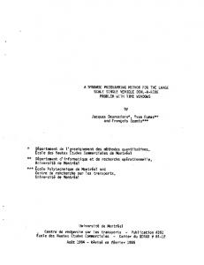
Figure 2: Search lattice for the rule-driven decoder. The gray circles indicated partial hypotheses. An hypothesis is expanded by applying an edge. DP recombination is used to restrict the search space throughout the rule lattice.

re-order rules. Additionally, rule-based probabilities can be used as well. This concept allows to directly compare a window-based decoder and the current rule based decoder in Section 5. The search space for the rule-driven decoder is illustrated in Fig. 2. The gray shaded circles represent translation hypotheses according to Eq. 4. A translation hypothesis h1 is extended by an edge which covers some uncovered portion of the input sentence to produce a new hypothesis h2 . The decoder searches monotonically through the entire chart of edges, and word re-ordering is possible only through the use of rule edges. The top half of the picture shows the way simple edges contribute to the search process: they are used to carry out a monotone translation. The dashed arrows indicate that hypotheses can be recombined: when extending hypothesis h3 by edge e = 2 and hypothesis h4 by edge e = 8 only a single hypothesis h5 is kept as the history of edge extensions can be ignored for future decoder decisions with respect to the uncovered source positions. Here, the distortion model and the language model history are ignored for illustration purposes. As it can be seen in Fig. 2, the rule edge generation step has created 3 copies of the simple edge e = 7, 41

which are marked by a dashed borderline. Hypotheses covering the same input may not be merged, i.e. hypotheses h9 and h13 for rules r = 1 and r = 2 have to be kept separate from the hypothesis h4 . But state merging may occur for states generated by rule edges for the same rule r, i.e. rule r = 1 and state h9 . Since rule edges have to be processed in a sequential order, looking up those that can extend a given hypothesis h is more complicated than a phrase translation look-up in a regular decoder. Given the search state definition in Eq. 4, for a given rule id r and coverage position s we have to be able to lookup all possible edge extensions efficiently. This is implemented by storing two lists: 1. For each source position j a list of possible ’starting’ edges: these are all the simple edges plus all rule edges with relative edge position p = BEG. This list is used to expand hypotheses according to the definition in Eq. 4 where the rule flag e = true, i.e. the search has finished covering an entire rule interval. 2. The second list is for continuing edges (p = INTER or p = END). For each rule id r, rule

start position sr and source position j a list of rule edges has to be stored that can continue an already started rule coverage. This list is used to expand hypotheses for which the rule flag e is e = false, i.e. the hypothesis has not yet finished covering the current rule interval, e.g. the hypotheses h9 and h11 in Fig. 2. The two lists are computed by a single run over the chart after all chart edges have been generated and before the search is carried out (the CPU time to generate these lists is included in the edge generation CPU time reported in Section 5). The two lists are used to find the successor edges for each hypothesis h that corresponds to a rule r efficiently: only a small fraction of the chart edges starting at position j needs to be retrieved for an extension. The rule start position sr has to be included for the second list: it is possible that the same rule r matches the input sentences for two intervals [i, j] and [i′ , j ′ ] which overlap. This results in an invalid search state configuration. Based on the two lists a monotone search is carried out over the extended rule edge set which implicitly generates a reordering lattice as in similar approaches (Crego and Marino, 2006; Zhang et al., 2007). But because the handling of the edges is tightly integrated into the beam search algorithm by applying the same beam thresholds it potentially handles 10’s of thousands of rules efficiently.

4

DP Search

The DP decoder described in the previous section bears some resemblance with search algorithms for large vocabulary speech recognition. For example, (Jelinek, 1998) presents a Viterbi decoder that searches a composite trellis consisting of smaller HMM acoustic trellises that are combined with language model states in the case a trigram language model. Multiple ’copies’ of the same acoustic sub models are incorporated into the overall trellis. The highest probability word sequences is obtained using a Viterbi shortest path finding algorithm in a possibly huge composite HMM (cf. Fig. 5.3 of (Jelinek, 1998)). In comparison, in this paper the edge ’copies’ are used to generate hypotheses that are hypotheses ’copies’ of the same phrase match, e.g. in Fig. 2 the states h4 , h8 , and h14 all result from covering the same simple edge e7 as the most 42

recent phrase match. The states form a potentially huge lattice as shown in Fig. 2. Similarly, (Ortmanns and Ney, 2000) presents a DP search algorithm where the interdependent decisions between non-linear time alignment, word boundary detection, and word identification (the pronunciation lexicon is organized efficiently as a lexical tree) are all carried out by searching a shortest path trough a possibly huge composite trellis or HMM. The similarity between those speech recognition algorithms and the current rule decoder derives from the following observation: the use of a language model in speech recognition introduces a coupling between adjacent acoustic word models. Similarly, a rule match which typically spans several source phrase matches introduces a coupling between adjacent simple edges. Viewed in this way, the handling of copies is a technique of incorporating higher-level knowledge sources into a simple one-step search process: either by processing acoustic models in the context of a language model or by processing simple edges in the context of bigger re-ordering units, which exploit a richer linguistic context. The Earley parser in the presentation (Jurafsky and Martin, 2000) also uses the notion of edges which represent partial constituents derived in the parsing process. These constituents are interpreted as edges in a directed acyclic graph (DAG) which represents the set of all sub parse trees considered. This paper uses the notion of edges as well following (Tillmann, 2006) where phrase-based decoding is also linked to a DAG path finding problem. Since the re-order rules are not applied recursively, the rule-driven algorithm can be linked to an Earley parser where parsing is done with a linear grammar (for a definition of linear grammar see (Harrison, 1978)). A formal analysis of the rule-driven decoder might be important because of the following consideration: in phrase-based machine translation the target sentence is generated from left-to-right by concatenating target phrases linked to source phrases that cover some source positions. Here, a coverage vector is typically used to ensure that each source position is covered a limited number of times (typically once). Including a coverage vector C into the search state definition results in an inherently exponential complexity: for an input sentence of length J there are 2J coverage vectors (Koehn, 2004). On

Table 2: Translation results on the MT06 data. w is the distortion limit.

Baseline decoder

Rule decoder (w = 15)

w=0 w=2 w=5 N (r) ≥ 2 N (r) ≥ 5

words / sec 171.6 25.4 8.2 9.1 10.5

the contrary, the search state definition in Eq. 4 explicitly avoids the use of a coverage vector resulting in an essentially linear time decoding algorithm (Section 5 reports the size of the the extended search graph in terms of number of edges and shows that the number of permutations per POS sequence is less than 2 on average). The rule-driven algorithm might be formally correct in the following sense. A phrase-based decoder has to generate a phrase alignment where each source position needs to be covered by exactly one source phrase. The rule-based decoder achieves this by local computation only: 1) no coverage vector is used, 2) the rule edge generation is local to each individual rule, i.e. looking only at the span of that rule, and 3) rules whose application spans overlap arbitrarily (but not recursively) are handled correctly. In future, a formal correctness proof might be given.

5

Experimental Results

We test the novel edge generation algorithm on a standard Arabic-to-English translation tasks: the MT06 Arabic-English DARPA evaluation set consisting of 1 529 sentences with 58 331 Arabic words and 4 English reference translations . The translation model is defined in Eq. 1 where 8 probabilistic features (language, translation,distortion model) are used. The distortion model is similar to (AlOnaizan and Papineni, 2006). An on-line algorithm similar to (Tillmann and Zhang, 2008) is used to train the weight vector w. The decoder uses a 5gram language model , and the phrase table consists of about 3.2 million phrase pairs. The phrase table as well as the probabilistic features are trained on a much larger training data consisting of 3.8 million sentences. Translation results are given in terms of the automatic BLEU evaluation metric (Papineni et al., 2002) as well as the TER metric (Snover et al., 43

generation [%] 1.90 0.29 0.10 0.75 0.43

BLEU 34.6 36.6 35.0 37.1 37.2

PREC 35.2 37.7 36.1 38.2 38.2

TER 65.3 63.5 65.1 63.5 63.5

2006). Our baseline decoder is similar to (Koehn, 2004; Moore and Quirk, 2007). The goal of the current paper is not to demonstrate an improvement in decoding speed but show the validity of the rule edge generation algorithm. While the baseline and the rule-driven decoder are compared with respect to speed, they are both run with conservatively large beam thresholds, e.g. a beam limit of 500 hypotheses and a beam threshold of 7.5 (logarithmic scale) per source position j. The baseline decoder and the rule decoder use only 2 stacks to carry out the search (rather than a stack for each source position) (Tillmann, 2006). No rest-cost estimation is employed. For the results in line 2 the number of phrase ’holes’ n in the coverage vector for a left to right traversal of the input sentence is restricted using a typical skip-based decoder (Berger et al., 1996). Up to 2 phrases can be skipped. Additionally, the phrase re-ordering is restricted to take place within a given window size w. The 28, 878 rules used in this paper are obtained from 14 989 manually aligned ArabicEnglish sentences where the Arabic sentences have been segmented and POS tagged . The rule selection procedure is similar to the one used in (Crego and Marino, 2006) and rules are extracted that occur at least twice. The rule-based re-ordering uses an additional probabilistic feature which is derived from the rule unigram count N (r) shown in Table. 1: p(r) = PNN(r) . The average number of POS se(r ′ ) r′

quence matches per input sentence is 34.9 where the average number of permutations that generate edges is 57.7. The average number of simple edges i.e. phrase pairs per input sentence is 751.1. For the rule-based decoder the average number of edges is 3187.8 which includes the simple edges. Table 2 presents results that compare the baseline decoder with the rule-driven decoder in terms

44

0.39 rule-driven decoder N(r)>=5 rule-driven decoder N(r)>=2 distortion-limited phrase decoder

0.38

BLEU

0.37 0.36 0.35 0.34 0.33 0

2

4

6

8

10

12

14

16

maximum window size

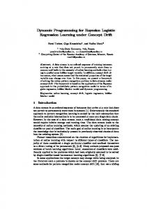
Figure 3: BLEU score as a function of window size w.

rule-driven decoder N(r)>=5 rule-driven decoder N(r)>=2 distortion-limited phrase decoder

100 CPU [words / sec]

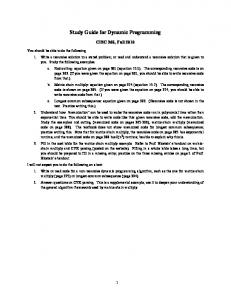
of translation performance and decoding speed. The second column shows the distortion limit used by the two decoders. For the rule-based decoder a maximum distortion limit w is implemented by filtering out all the rule matches where the size of the rule in terms of number of POS symbols is greater than w, i.e. the rule edges are processed monotonically but a monotone rule edge sequence for the same rule id may not span more than w source positions. The third column shows the translation speed in terms of words per second. The fourth column shows the percentage of CPU time needed for the edge generation (including both simple and rule edges). The final three columns report translation results in terms of BLEU , BLEU precision score (PREC), and TER. The rule-based reordering restriction obtains the best translation scores on the MT06 data: a BLEU score of 37.2 compared to a BLEU score of 36.6 for the baseline decoder. The statistical significance interval is rather large: 2.9 % on this test set as text from various genres is included. Additional visual evaluation on the dev set data shows that some successful phrase reordering is carried out by the rule decoder which is not handled correctly by the baseline decoder. As can be seen from the results reducing the number of rules by filtering all rules that occur at least 5 times (about 10 000 rules) slightly improves translation performance from 37.1 to 37.2. The edge generation accounts for only a small fraction of the overall decoding time. Fig. 3 and Fig. 4 demonstrate additional advantages when using the rule-based decoder. Fig. 3 shows the translation BLEU score as a function of the distortion limit window w. The BLEU score actually decreases for the baseline decoder as the size w is increased. The optimal window size is surprisingly small: w = 2. A similar behavior is also reported in (Moore and Quirk, 2007) where w = 5 is used . For the rule-driven decoder however the BLEU score does not decrease for large w: the rules restrict the local re-ordering in the context of potentially very long POS sequences which makes the re-ordering more reliable. Fig. 4 which shows the decoding speed as a function of the window size w demonstrates that the rule-based decoder actually runs faster than the baseline decoder for window sizes w ≥ 5.

10

0

2

4

6

8

10

12

14

16

maximum window size

Figure 4: Decoding speed as a function of window size w.

6

Discussion and Future Work

The handling of the re-order rules is most similar to work in (Crego and Marino, 2006) where the rules are used to create re-order lattices. To make this feasible, the rules have been vigorously filtered in (Crego and Marino, 2006): only about 30 rules are used in their experiments. On the contrary, the current approach tightly integrates the re-order rules into a phrase-based decoder such that 29 000 rules can be handled efficiently. In future work our novel approach might allow to make use of lexicalized reorder rules as in (Xia and McCord, 2004) or syntactic rules as in (Wang et al., 2007).

7

Acknowledgment

This work was supported by the DARPA GALE project under the contract number HR0011-06-200001. The authors would like to thank the anonymous reviewers for their detailed criticism.

References Yaser Al-Onaizan and Kishore Papineni. 2006. Distortion Models for Statistical Machine Translation. In Proceedings of ACL-COLING’06, pages 529–536, Sydney, Australia, July. Adam L. Berger, Peter F. Brown, Stephen A. Della Pietra, Vincent J. Della Pietra, Andrew S. Kehler, and Robert L. Mercer. 1996. Language Translation Apparatus and Method of Using Context-Based Translation Models. United States Patent, Patent Number 5510981, April. David Chiang. 2007. Hierarchical Machine Translation. Computational Linguistics, 33(2):201–228. Michael Collins, Philipp Koehn, and Ivona Kucerova. 2005. Clause restructuring for statistical machine translation. In Proc. of ACL’05, pages 531–540, Ann Arbor, Michigan, June. Association for Computational Linguistics. J.M. Crego and Jos´e B. Marino. 2006. Integration of POStag-based Source Reordering into SMT Decoding by an Extended Search Graph. In Proc. of AMTA06, pages 29–36, Cambridge, MA, August. Jay Earley. 1970. An Efficient Context-Free Parsing Algorithm. Communications of the ACM, 13(2):94–102. Michael A. Harrison. 1978. Introduction to Formal Language Theory. Addison Wesley. Fred Jelinek. 1998. Statistical Methods for Speech Recognition. The MIT Press, Cambridge, MA. Daniel Jurafsky and James H. Martin. 2000. Speech and Language Processing. Prentice Hall. Philipp Koehn, Franz J. Och, and Daniel Marcu. 2003. Statistical phrase-based translation. In HLTNAACL’03: Main Proceedings, pages 127–133, Edmonton, Alberta, Canada, May 27 - June 1. Philipp Koehn. 2004. Pharaoh: a Beam Search Decoder for Phrase-Based Statistical Machine Translation Models. In Proceedings of AMTA’04, Washington DC, September-October. Robet C. Moore and Chris Quirk. 2007. Faster Beamsearch Decoding for Phrasal SMT. Proc. of the MT Summit XI, pages 321–327, September. Masaaki Nagata, Kuniko Saito, Kazuhide Yamamoto, and Kazuteru Ohashi. 2006. A Clustered Global Phrase Reordering Model for Statistical Machine Translation. In Proceedings of ACL-COLING’06, pages 713–720, Sydney, Australia, July. Franz-Josef Och and Hermann Ney. 2004. The Alignment Template Approach to Statistical Machine Translation. Computational Linguistics, 30(4):417–450. Stefan Ortmanns and Hermann Ney. 2000. Progress in Dynamic Programming Search for LVCSR. Proc. of the IEEE, 88(8):1224–1240.

45

Kishore Papineni, Salim Roukos, Todd Ward, and WeiJing Zhu. 2002. BLEU: A Method for Automatic Evaluation of Machine Translation. In Proc. of ACL’02, pages 311–318, Philadelphia, PA, July. Matthias Paulik, Kay Rottmann, Jan Niehues, Silja Hildebrand, and Stephan Vogel. 2007. The ISL Phrase-Based MT System for the 2007 ACL Workshop on SMT. In Proc. of the ACL 2007 Second Workshop on SMT, June. Matthew Snover, Bonnie Dorr, Richard Schwartz, Linnea Micciulla, and John Makhoul. 2006. A Study of Translation Edit Rate with Targeted Human Annotation. In Proc. of AMTA 2006, Boston,MA. Christoph Tillmann and Tong Zhang. 2007. A Block Bigram Prediction Model for Statistical Machine Translation. ACM-TSLP, 4(6):1–31, July. Christoph Tillmann and Tong Zhang. 2008. An Online Relevant Set Algorithm for Statistical Machine Translation. Accepted for publication in IEEE Transaction on Audio, Speech, and Language Processing. Christoph Tillmann. 2006. Efficient Dynamic Programming Search Algorithms for Phrase-based SMT. In Proceedings of the Workshop CHPSLP at HLT’06, pages 9–16, New York City, NY, June. Chao Wang, Michael Collins, and Philipp Koehn. 2007. Chinese Syntactic reordering for statistical machine translation. In Proc. of EMNLP-CoNLL’07, pages 737–745, Prague, Czech Republic, July. Fei Xia and Michael McCord. 2004. Improving a statistical mt system with automatically learned rewrite patterns. In Proc. of Coling 2004, pages 508–514, Geneva, Switzerland, Aug 23–Aug 27. COLING. Yuqi Zhang, Richard Zens, and Hermann Ney. 2007. Chunk-level Reordering of Source Language Sentences with Automatically Learned Rules for Statistical Machine Translation. In Proc. of SSST, NAACLHLT’07 / AMTA Workshop, pages 1–8, Rochester, NY, April.