c o m p u t e r m e t h o d s a n d p r o g r a m s i n b i o m e d i c i n e 8 9 ( 2 0 0 8 ) 50–55
journal homepage: www.intl.elsevierhealth.com/journals/cmpb
A SAS program for calculating cumulative incidence of events (with confidence limits) and number at risk at specified time intervals with partially censored data Alan D. Penman a,∗ , W.D. Johnson b a
Department of Medicine, University of Mississippi Medical Center, Clinical Research Program (Building LK), 876A Lakeland Drive, Jackson, MS, United States b Department of Preventive Medicine, University of Mississippi Medical Center, Jackson, MS, United States
a r t i c l e
i n f o
a b s t r a c t
Article history:
Correct analysis and interpretation of longitudinal (cohort) studies with partially censored
Received 10 February 2007
time-to-event data requires that the cumulative count of events and censored observa-
Received in revised form
tions as well as the number at risk be calculated at appropriate time points (for example,
17 July 2007
every year), by baseline group or stratum. We present here a simple SAS program, for use
Accepted 8 October 2007
in situations in which competing risks do not need to be accounted for, that calculates, by baseline group or stratum, the cumulative event count, cumulative event probabil-
Keywords:
ity (with upper and lower 95% confidence limits), and number at risk at selected time
Survival data
points that can be chosen by the user. We demonstrate the use of the program in the
Cumulative incidence
analysis of longitudinal time-to-event data from a prospective study, the Atherosclero-
Number at risk
sis Risk In Communities (ARIC) Study, for four groups and a 10-year follow-up. The SAS code presented here is easy to follow and modify and can be incorporated quickly by the user for immediate use. It provides an especially valuable tool for less experienced SAS users. © 2007 Elsevier Ireland Ltd. All rights reserved.
1.
Introduction
In longitudinal (cohort) studies with time-to-event data a main outcome measure of interest is an estimate of the cumulative incidence probability (where the incidence probability is 1—survival probability). This may be presented in crude (unadjusted) form or, if comparisons are to be made with an external standard or among baseline groups (or strata), adjusted for baseline group differences in age, sex, race, or other covariates. The Kaplan–Meier product-limit method is used to estimate the unadjusted cumulative incidence probability, [1] and Cox proportional hazards regression is used to
∗
estimate the adjusted cumulative incidence probability by various methods [2–4]. The results of both methods are usually presented graphically with an appropriate time scale on the Xaxis. Correct interpretation of these graphs, and, in particular, of group differences in the incidence curves, requires that the number at risk in each baseline group be displayed at appropriate time points, for example, every year [5]. We present here a simple SAS program that, in situations in which competing risks do not need to be accounted for, calculates the cumulative event count, cumulative event probability (with upper and lower 95% confidence limits), and number at risk at selected time points that can be chosen by the user.
Corresponding author. Tel.: +1 601 815 5836; fax: +1 601 815 1332. E-mail address:
[email protected] (A.D. Penman). 0169-2607/$ – see front matter © 2007 Elsevier Ireland Ltd. All rights reserved. doi:10.1016/j.cmpb.2007.10.004
51
c o m p u t e r m e t h o d s a n d p r o g r a m s i n b i o m e d i c i n e 8 9 ( 2 0 0 8 ) 50–55
Table 1 – Endpoint frequencies by follow-up time interval—first quartile Follow-up time interval (years)
0–1 1–2 2–3 3–4 4–5 5–6 6–7 7–8 8–9 9–10 >10 years Total
2.
Endpoint frequencies Number of events
Number of censored observations
0 2 1 1 2 0 3 4 1 0 0
3 2 4 2 4 4 4 49 164 136 62
3 4 5 3 6 4 7 53 165 136 62
14
434
448
The SAS program
The following program, written in SAS Version 9.1, [6] has three sections. The first section produces numbers of events and censored observations by time interval. The second section produces cumulative frequencies and number at risk at each time point. The third section produces cumulative incidence probabilities, with upper and lower 95% confidence limits, again by time interval. We have written the program for four baseline groups and a 10-year follow-up, but it can be easily modified by straightforward addition or deletion of code to analyze data with any number of baseline groups and any length of follow-up. The program makes minimum use of SAS macro coding, plus (in Section 2) some SAS output delivery system (ODS) code. The following macro-variables should be set by the user: 1. In Section 1, the dataset name, the name of the variable for follow-up time, the name of the censoring variable, and the name of the grouping (or stratum) variable, thus: %macro section1 (name, time, event, group); 2. In Section 2, the number of groups (strata), the dataset name, the name of the grouping (or stratum) variable, and the number of subjects in each group (stratum), thus: %macro section2 (numgrps, name, group, grpnum1, grpnum2, grpnum3, grpnum4); 3. In Section 3: the dataset name and the name of the grouping (or stratum) variable, thus: %macro section3 (name, group). These are the only pieces of information required for the user. Of course, if a permanent dataset is being used the macros must be preceded by a LIBNAME statement to indicate path/folder. The complete SAS program is given in Appendix A.
3.
Total
Example
We demonstrate the use of the program in the analysis of longitudinal time-to-event data from the Atherosclero-
sis Risk in Communities (ARIC) Study, a prospective study, begun in 1987, designed to investigate the etiology and natural history of cardiovascular disease (CVD) in four U.S. communities. The study design and procedures have been reported previously [7]. At the Jackson field center (Mississippi) only African-Americans were recruited. During the third ARIC examination (1993–1995), echocardiographic examination was performed at the Jackson field center on 2445 middle-aged and elderly African-American men and women, 51–70 years of age. Of these 2445 participants, 1792 had an adequate Mmode echocardiogram for assessing left ventricular mass and were free from prevalent stroke, left ventricular aneurysm, aortic stenosis, and mitral stenosis. The aim of the analysis was to determine the association between echocardiographically defined indexed left ventricular mass (LVMI), in quartiles, and the incidence of first stroke [8]. This dataset (dataset1) includes variables for follow-up time (ISCstrfuyrs), censoring status (IN03ISC), and group (LVMIQUARTILE) with four levels (n = 448 persons in each). The macros are run with these user-defined parameters: • %section1 (dataset1, ISCstrfuyrs, IN03ISC, LVMIQUARTILE); • %section2 (4, dataset1, LVMIQUARTILE, 448, 448, 448, 448); • %section3 (dataset1, LVMIQUARTILE).
Table 2 – Cumulative frequency of endpoints and number at risk in each time interval—first quartile Follow-up time interval (years) 0–1 1–2 2–3 3–4 4–5 5–6 6–7 7–8 8–9 9–10 >10
Cumulative frequency of endpoints 3 7 12 15 21 25 32 85 250 386 448
Number at risk in each time interval 445 441 436 433 427 423 416 363 198 62 0
52
c o m p u t e r m e t h o d s a n d p r o g r a m s i n b i o m e d i c i n e 8 9 ( 2 0 0 8 ) 50–55
Table 3 – Cumulative incidence probabilities and 95% confidence limits—first quartile Duration of follow-up (years) 1 2 3 4 5 7 8 9
Cumulative incidence probability (%)
Lower 95% confidence limit
0.0 0.4 0.7 0.9 1.4 2.1 3.0 3.4
The complete SAS output consists of 12 tables:
1. Four tables (one per quartile) of numbers of events and censored observation by year; 2. Four tables (one per quartile) of cumulative frequency and number at risk year; 3. Four tables (one per quartile) of cumulative incidence probabilities, with upper and lower 95% confidence limits, by year.
To save space, only the three tables for the first quartile (modified slightly for clarity) are shown here. For each group (quartile), the number of events (new strokes) and censored observations by time period (year) are shown in Table 1 and the numbers at risk by time period (year) are shown in Table 2. The cumulative incidence probabilities by time period (year) are shown in Table 3. The cumulative incidence graph (Fig. 1) shows the number at risk in each group (quartile) in the footnote lines; as can be seen, the numbers for the first quartile are taken from Table 2.
0.0 0.1 0.2 0.3 0.6 1.1 1.8 2.0
4.
Upper 95% confidence limit 0.0 0.8 2.1 2.4 3.0 3.9 5.2 5.6
Discussion
A number of SAS macros for calculating cumulative incidence can be found on the Internet for public use (see, for example, [2–4] and [9]). They are usually more complicated and harder to follow, which may limit their adoption. The SAS code presented here is easy to follow and modify and can be incorporated quickly by the user for immediate use. It provides an especially valuable tool for less experienced SAS users. A particularly useful output from this program, in our view, is the table of number at risk in each group, by time interval. This is not produced by any of the survival analysis procedures in SAS (PROC LIFETEST, PROC LIFEREG); it can be calculated by hand using the routine output but this can be tedious to do. Correct interpretation of survival plots requires this information, [5] and more and more journals now ask for it. One slight limitation of the program is that no table row is created for time points without events or censored observations; for example, in Table 3, which shows the cumulative incidence probabilities for the first quartile, the row entry for
Fig. 1 – Cumulative stroke incidence curves (by LVMI quartile).
c o m p u t e r m e t h o d s a n d p r o g r a m s i n b i o m e d i c i n e 8 9 ( 2 0 0 8 ) 50–55
time 6 years is missing (as well as row entries for follow-up times greater than 9 years) because there were no events in that time period. This should be kept in mind when the data are being copied into a figure. Our program has been written for four baseline groups and a 10-year follow-up, but it can be easily modified by straightforward addition or deletion of code to analyze data with any number of baseline groups and any length of followup. We have also assumed that follow-up time has been recorded in years (which is then converted in Section 1 into months). However, if in the original dataset follow-up time
53
has been recorded in months, this conversion step can easily be skipped. It should be remembered that in situations in which competing risks need to be accounted for conventional Kaplan–Meier procedures overestimate the cause-specific cumulative incidence probabilities [9,10]. Use of this SAS macro is best reserved for the analysis of overall cumulative incidence probabilities (such as overall mortality/survival or overall event probabilities).
Appendix A. SAS CODE
54
c o m p u t e r m e t h o d s a n d p r o g r a m s i n b i o m e d i c i n e 8 9 ( 2 0 0 8 ) 50–55
c o m p u t e r m e t h o d s a n d p r o g r a m s i n b i o m e d i c i n e 8 9 ( 2 0 0 8 ) 50–55
references
[1] The LIFETEST Procedure. SAS OnlineDoc 9.1.3. SAS Institute, Cary, NC. Available at: http://support.sas.com/onlinedoc/913/docMainpage.jsp (last accessed July 16, 2007). [2] W.A. Ghali, H. Quan, R. Brant, G. van Melle, C.M. Norris, P.D. Faris, P.D. Galbraith, M.L. Knudtson, Comparison of two methods for calculating adjusted survival curves from proportional hazards models, JAMA 286 (12) (2001) 1494–1497. [3] J. Lee, C. Yoshizawa, L. Wilkens, H.P. Lee, Covariance adjustment of survival curves based on Cox’s proportional hazards regression model, Comput. Appl. Biosci. 8 (1) (1992) 23–27. [4] F.J. Nieto, J. Coresh, Adjusting survival curves for confounders: a review and a new method, Am. J. Epidemiol. 143 (10) (1996) 1059–1068.
55
[5] S.J. Pocock, T.C. Clayton, D.G. Altman, Survival plots of time-to-event outcomes in clinical trials: good practice and pitfalls, Lancet 359 (9318) (2002) 1686–1689. [6] SAS Institute, Cary, NC, 2007. [7] A.R.I.C. The, Investigators, The Atherosclerosis Risk in Communities (ARIC) Study: design and objectives, Am. J. Epidemiol. 129 (4) (1989) 687–702. [8] E.R. Fox, N. Alnabhan, A. Penman, et al., Echocardiographic left ventricular mass index predicts incident stroke in African-Americans: the Atherosclerosis Risk in Communities (ARIC) Study, Stroke 38 (2007) 2686–2691. [9] S. Rosthoj, P.K. Andersen, S.Z. Abildstrom, SAS macros for estimation of the cumulative incidence functions based on a Cox regression model for competing risks survival data, Comput. Methods Programs Biomed. 74 (1) (2004) 69–75. [10] J.M. Satagopan, L. Ben-Porat, M. Berwick, M. Robson, D. Kutler, A.D. Auerbach, A note on competing risks in survival data analysis, Br. J. Cancer 91 (2004) 1229–1235.