A SAT-based Decision Procedure for the Boolean

A SAT-based Decision Procedure for the Boolean Combination of Difference Constraints Alessandro Armando, Claudio Castellini, Enrico Giunchiglia, and Marco Maratea MRG-DIST, University of Genova viale Francesco Causa, 13 — 16145 Genova (Italy) {armando, drwho, enrico, marco}@mrg.dist.unige.it

Abstract. The problem of solving boolean combinations of difference constraints is at the core of many important techniques such as planning, scheduling, and model-checking of real-time systems. Efficient decision procedures for this class of formulas are, therefore, strongly needed. In this paper we present TSAT++, a SAT-based open reasoning platform able to decide boolean combinations of difference constraints. Experimental results indicate that TSAT++ outperforms its competitors both on randomly-generated, hand-made and real world problems.

1 Introduction Decision procedures for the boolean combination of difference constraints, i.e. constraints of the form x − y ≤ c where x and y are variables ranging over a fixed numeric domain (typically the integers or the reals) and c is a constant in the same domain, play a pivotal role in many important techniques such as planning, scheduling, and model-checking of real-time systems. In the last 5 years, at least 6 systems have been proposed that are able to deal with disjunctions of difference constraints, 4 of which in the AI literature and 2 in the formal verification literature, meaning that the topic is hot and interdisciplinary. Of these 6 systems, 5 are SAT-based or CSP-based. This means that the satisfiability of a problem φ is determined by 1. generating a set of propositional atoms and difference constraints “propositionally satisfying” φ, using SAT or CSP techniques, and 2. testing the consistency of each generated set using standard techniques (such as, e.g., the Bellman-Ford procedure). As we will see, of fundamental importance is the generation step, and thus the specific SAT/CSP techniques being used. Despite of this, none of these 5 systems take advantage of the recent developments in the SAT field. In this paper we present TSAT++, an open reasoning platform able to deal with propositional atoms and arbitrary conjunctions, disjunctions, and negations of difference constraints. TSAT++ integrates the latest techniques proposed in the SAT field (and, in particular, those proposed in [10]) and proposes new ideas designed to take maximum advantage from the techniques used in the generation phase. Because of these new methods and their fruitful integration, TSAT++ has a clear edge over its competitors: An extensive comparative analysis, involving all the above mentioned 6 systems, on randomly generated, hand-made and real world problems, shows that TSAT++ (i) on randomly generated problems, in the hard region is at least 2 orders of magnitude (resp. a factor of 6) faster if variables range over the reals (resp. the integers); (ii) on instances coming from real world problems, is on average at least a factor of 4 faster; and (iii) on handmade problems, is up to 3 orders of magnitude faster than its fastest competitor in each category. These results are significant, especially if one considers that, contrarily to some of its competitors, TSAT++ is not tuned nor customized on any particular class of problems. The paper is structured as follows. First, we give the definitions necessary for the rest of the paper. Then we present the ideas implemented in TSAT++ and the experimental results. Lastly, some conclusions are drawn.

A SAT-based Decision Procedure for the Boolean Combination of Difference Constraints

167

2 Preliminaries Let V and P be two disjoint sets of symbols, called variables and propositional atoms respectively. A difference constraint is an expression of the form x − y ≤ c where x, y ∈ V and c is a numeric constant. An atom is either a difference constraint or a propositional atom; a literal is either an atom or its negation. If a is an atom, then a abbreviates ¬a and ¬a stands for a. Lastly, a Temporal Reasoning Problem (TRP) is a Boolean combination of atoms. Thus, our logic is as expressive as Separation Logic [14], which allows also for , =, and 6=, but which can be easily expressed in our formalism. Another well-known formalism in this area is the Disjunctive Temporal Logic, which allows only for formulas in CNF whose literals are restricted to be difference constraints. Formulas of Disjunctive Temporal Logic are called Simple Temporal Problems. In order to define the semantics of a TRP we need first to fix a domain D (of interpretation) for the variables: The possible candidates are the set of real numbers or the set of integers. An assignment is a function mapping each variable to an element of D, and each propositional atom to the truth values {⊥, ⊤}. An assignment σ is extended to map a TRP to {⊥, ⊤} by defining – σ(x − y ≤ c) = ⊤ if and only if σ(x) − σ(y) ≤ c, and – σ(φ) = ⊤ (with φ being a TRP) according to the truth tables of propositional logic. Let φ be a TRP. We say that an assignment σ satisfies φ if and only if σ(φ) = ⊤. φ is satisfiable (consistent) (in D) if and only if there exists an assignment (on D) which satisfies it. A finite set of literals is satisfiable (consistent) (in D) if and only if their conjunction, as a TRP, is. Here, we deal with the problem of determining whether a TRP is satisfiable or not in the fixed domain of interpretation. Clearly the problem is NP-complete, independently from whether D represents the integers or the reals. In the following, we will use the term valuation to mean a mapping from atoms to {⊥, ⊤}, extended to arbitrary TRPs according to the truth tables of propositional logic. We will represent a valuation as the set of literals assigned to true. We will refer to a satisfying assignment also as TRP-model. Further, we restrict our attention to TRPs in CNF. This is not a limitation since any TRP can be efficiently reduced to an equi-satisfiable formula in CNF. With this assumption, we represent a TRP as a set of clauses, each clause being a set of literals. TSAT++ is able to deal with any such TRP. The system presented in [13] (that we will call SK), Tsat [1], CSPi [11], and Epilitis [15] are restricted to problems in Disjunctive Temporal Logic (DTPs). TSAT++ is as expressive as SEP [14], and not comparable to MathSAT [2]: while MathSAT allows for arbitrary linear constraints as atoms, it does not allow to consider the integers as domain of interpretation.

3 SAT and CSP-based procedures With the exception of SEP, all the other 5 systems are quite similar from an algorithmic point of view. In fact, given a DTP φ, all such systems work by 1. (generation phase) generating all the valuations µ which satisfy φ, 2. (consistency checking) for each µ, testing whether the STP corresponding to µ is satisfiable. The generation phase can be done as search in a Constraint Satisfaction Problem (CSP) associated to the basic temporal reasoning problem (SK, CSPi, Epilitis) or by solving the corresponding propositional satisfiability problem (SAT) (Tsat, MathSAT, TSAT++). In the first approach, search is performed in a metasearch space in which a new variable is associated with each clause, its domain being the set of disjuncts in the clause. In the SAT-based approach, the given TRP is abstracted into a propositional formula obtained by substituting each distinct binary constraint with a newly introduced propositional atom. SAT and CSP-based approaches are tightly connected, and it is therefore not surprising that in their basic versions and starting from Tsat, all the systems perform the following steps: 1. assign to true the literals in unit clauses (a clause is unit if it has cardinality 1),1 2. if there are no more literals to assign according to the previous step, they branch on a literal l (i.e., assign true to l), and—upon the failure of the subsequent search—add the negation of l to the current state and continue the search, till either a satisfying assignment is found, or backtrack has to occur. The similarity to the search performed by SAT solvers is apparent. Despite of this, none of SAT and CSPbased systems incorporates the last advancements done in the SAT field. 1

In CSPi, Epilitis, the fact that unit clauses are assigned first is “hidden” in the heuristics used for selecting the literal to branch on. Further, these systems also employ forward checking, which removes binary constraints whose negation is entailed by the current valuation.

168

Alessandro Armando et al.

4 TSAT++ In this section, we describe the main ideas behind TSAT++, and in particular, (i) the computation done before the search starts (pre-processing), (ii) the way the search space is pruned after each branching node (look-ahead), (iii) the way recovery from failures happens (look-back); (iv) the heuristics used for picking the literal on which to branch (branching rule), and (v) the procedure used for checking the satisfiability of a set of literals (consistency checking). TSAT++ employs an API-like modified version of SIMO [7] for the generating phase. 4.1 Pre-processing One drawback of the generate-and-test approach is that (exponentially) many trivially inconsistent valuations can be generated and then discarded. This may happen both in SAT and CSP-based approaches given that, in the generation phase, there is no constraint relating the truth values of, e.g., x−y ≤ 3 and x−y ≤ 5. Thus, many trivially inconsistent valuations (e.g., with x − y ≤ 3 assigned to true and x − y ≤ 5 to false) can be generated. To reduce the generation of unfruitful valuations, in TSAT++ for each pair c1 , c2 of difference constraints in the same variables and occurring in the input formula, the consistency of all possible pairs of literals built out of them, i.e., {c1 , c2 }, {¬c1 , c2 }, {c1 , ¬c2 }, and {¬c1 , ¬c2 }, is checked, and, assuming, e.g., {c1 , c2 } is inconsistent, the clause {¬c1 , ¬c2 } is added to the input formula before the search starts. In our example, we would add the clause {¬x − y ≤ 3, x − y ≤ 5}. This dramatically speeds-up the search, especially on randomly generated problems. In fact, e.g., as soon as x − y ≤ 3 is assigned to true, x − y ≤ 5 gets also assigned to true by unit propagation. 4.2 Look-ahead Consider a TRP φ and let S be the set of literals assigned to true so far. The idea behind look-ahead techniques is to try to detect new literals l that are entailed by φ and S, i.e., such that l is satisfied by each assignment satisfying φ and S. If l is one of such literal, we can (i) add l to S and (ii) simplify φ on the basis that l is true. This has the beneficial effect of postponing the branching phase and in doing so it may lead to huge savings. The basic look-ahead technique common to all solvers is unit-propagation. A simple profiling of the code of TSAT++ on real-world problems reveals that most of the CPU time is spent in the generation phase (often more than 80%, sometime close to 100%), within which most of the time is spent by unit-propagation (> 90% in most cases). Therefore, the choice of a good data-structure for unit-propagation is capital. Two-literal watching is an efficient data-structure for unit-propagation (see, e.g., [10]). With it, each clause maintains two fields meant to store two “watched” open (i.e. not assigned) literals. Assigning an atom and detecting new units, causes the visit of a sub-linear (in the number of occurrences of the atom) number of clauses. Further, following [10], when backtracking occurs, nothing needs to be undone, and thus backtracking takes constant time. Notice that by using standard counters structures, as in, e.g., Tsat and MathSAT, assigning an atom and detecting new units has a cost which is at least linear in the number of occurrences of the atom. Furthermore when backtracking occurs and an atom is de-assigned, each operation done has to be undone and this again has a cost which is linear in the number of occurrences of the atom. 4.3 Look-back If recovery from a failure is performed by simple chronological backtracking, it is not infrequent to keep exploring a possibly large subtree whose leaves are all dead-ends, especially if the failure is due to some choices performed way up in the search tree. The solution to this problem is to jump back over the choices that do not belong to the reason for the failure. Intuitively, if S is a set of literals such that S ∪ φ (where φ is the input CNF formula) is unsatisfiable, then a reason R for S is a subset of S such that φ ∪ R is unsatisfiable. Reasons are initialized as soon as an inconsistency is detected, and updated while backtracking. The corresponding technique is known as (Conflict-Directed) Back-jumping (CBJ) [12]. With learning [3], each reason R computed while back-jumping is turned into the clause {l | l ∈ R} that may be added to the input formula. Learnt clauses will prune the subsequent search space, thus avoiding the repetition of the same

A SAT-based Decision Procedure for the Boolean Combination of Difference Constraints

169

mistakes. On the other hand, exponentially many reasons can be learnt, and each learnt clause causes an overhead when assigning literals. In practice it is necessary to introduce criteria (i) for limiting the clauses that have to be learnt or (ii) for removing some of them. TSAT++ features 1-UIP learning [10]. This technique ensures that at each decision level of each branch at most one clause is added to the input formula. Still, an exponential blow-up may happen. To prevent this in TSAT++, each added clauses is analyzed with a given periodicity and (possibly) deleted. Standard alternatives to 1-UIP learning are [3] 1. relevance-bounded learning of order n (used in MathSAT with n = 3, 4) and 2. size-bounded learning of order n (used in Epilitis with n = 10). Compared to the 1-UIP learning implemented in TSAT++, both MathSAT and Epilitis may store more than one clause per level. 4.4 Branching rule TSAT++ uses a conflict-based heuristic, whose basic idea is to select the literal mostly occurring in the most recently learnt clauses. The rationale behind it is that learnt clauses represent conflicts among the literals that have emerged during the search. By satisfying these clauses we avoid the repetition of the same mistake. However, not all the learnt clauses are equally important: Indeed, some of them, e.g., those discovered at the beginning of the search, may become obsolete for guiding the search in the current branch. Thus, the score associated with each literal is periodically divided by 2, giving more relevance to the atoms that will occur in the newly discovered conflicts. Of course, such conflict-based heuristics make sense only for solvers with learning. Epilitis uses a similar heuristics. The main difference is that, in Epilitis, all conflicts are equally important, i.e., it does not focus on the atoms in the most recently learnt clauses. MathSAT employs a wide variety of heuristics, some of which specifically designed for solving a specific class of problems. However, even though MathSAT uses learning and thus could employ a conflict-based heuristic, all its heuristics are MOMS-based (Maximum Occurrences in clauses of Minimal Size): They give higher scores to literals in shorter clauses. These heuristics have been mutuated from the SAT literature, and are used also by Tsat. In the CSP-based systems, MOMS-based heuristics correspond to the Minimum Remaining Value (MRV) heuristics, used in SK and CSPi. 4.5 Consistency checking Consider a set S of literals. For all the procedures here considered, an effective method for checking the consistency of S is needed. Moreover, when S is unsatisfiable, it is important to be able to extract a reason of its unsatisfiability, i.e., an unsatisfiable subset S ′ of S. Of course, a very fast selection of such a set S ′ is the set S itself. However applying this selection is seldom a good idea since S ′ is to be used by the lookback mechanisms, e.g., to backjump over irrelevant nodes. It is thus of fundamental importance to keep S ′ as “small” as possible in order to try to maximize the benefits of the look-back. We now describe how we compute such a small set S ′ . For the time being, let us assume that S is just a set of difference constraints, i.e., that we are facing a STP. We will see later how to generalize the discussion to arbitrary literals. The standard method to check the consistency of a STP S, is the BellmanFord procedure (BF), see, e.g., [4]. The basic idea is to associate with S a constraint graph, whose nodes are the variables in S, and which has an edge from y to x with weight c, for each constraint x − y ≤ c in S. Then, an extra node s (the “source”) connected to all the other nodes with weight 0 is added, and BF is used to compute the “single source shortest-paths” problem. If S is consistent, there are no negative cycles in the graph, and BF returns true. Otherwise, it is easy to modify BF to return a minimal (under a given set property) subset S ′ of S which is inconsistent. The first observation is that the constraint graph of S may have several different negative cycles, each corresponding to a minimal inconsistent subset of S. The standard approach amounts to stopping the search as soon as one such negative cycle is detected. TSAT++ instead continues the search in order to determine a negative cycle involving the smallest possible number of nodes (corresponding to an inconsistent set with minimal cardinality). This modification does not alter the overall complexity of BF, which remains O(n × m), where n and m are the numbers of variables and constraints in S respectively. The second observation is that, when S is a valuation satisfying the input TRP φ, it may be the case that some of the

170

Alessandro Armando et al.

literals in S may be not necessary to satisfy φ. In other words, there may be a literal l in S such that, for each clause C ∈ φ with l ∈ C, there is another literal l′ in S ∩ C. If this is the case, also (S \ {l}) ∪ {l} satisfies φ, and we can safely check the consistency of S \ {l} instead of S. TSAT++ may recursively eliminate such literals l from S, assuming l is a difference constraint or the negation thereof. If S ′ ⊆ S is the resulting set, it will then check the satisfiability of S ′ . We call the above procedure reduction, and it may be useful because – if S is satisfiable, so is S ′ , and we are done; – if S is unsatisfiable, it may nevertheless be the case that S ′ is satisfiable, and we can still interrupt the search and exit with a satisfying assignment; – if S and S ′ are both unsatisfiable, checking the consistency of S instead of S ′ can cause exponentially many more consistency checks. In fact, any valuation extending S ′ also satisfies φ, and each could be generated and then rejected by TSAT++. The last two cases are of particular relevance in TSAT++. In fact, because of the two-literal watching data structure, the generated valuations satisfying φ are always total. Thus, it is very often the case that huge portions of the difference constraints in S are irrelevant for satisfying φ and, by removing them, we end-up in a set S ′ with many less difference constraints. Notice that the reduction procedure is not to be applied when early pruning is enabled. With early pruning, the hope is that S is unsatisfiable in order to stop the search. If S ′ turns out to be satisfiable, we cannot conclude about S, and we have to go on expanding S. So far, we have been using the assumption that S is a set of difference constraints. The problem is how to deal with the negation of difference constraints. Assume we have ¬x − y ≤ c in S. Then, such a literal is equivalent to y − x < −c, and we can replace every such constraint in S with a constraint y − x ≤ d, where d is – the maximum integer strictly smaller than −c, if variables range over the integers; and – −c − 10p (n12 +1) , otherwise. In the expression, n is the number of variables in S, and p is the maximum number of digits appearing to the right of the decimal point (assuming that there are no useless “0”), in any of the constants of the input TRP. If all the constants are integers, p = 0. The resulting set does not contain any negation of difference constraint, and it is satisfiable if and only if the initial set is (this follows from Theorem 3 in [6]).

5 Experimental Analysis 5.1 Experimental setting In order to thoroughly compare TSAT++, we have considered a wide variety of publicly available random, handmade, and real-world TRPs (the classification has been done following what is standard practice in the SAT competition [8]). As for the solvers, we have initially considered all the publicly available systems, namely SK, CSPi, Epilitis, MathSAT, SEP, and Tsat plus—of course—TSAT++. After a first run, we have discarded SK, because clearly non competitive with respect to the others. Each solver has been run on all the benchmarks it can deal with, not only on the benchmarks the solver was analyzed on by the authors. In particular, Epilitis can only handle DTPs with binary clauses and integer valued variables; CSPi and Tsat can only handle DTPs with real valued variables; MathSAT can handle arbitrary TRPs with real valued variables; SEP and TSAT++ can handle arbitrary TRPs. Each solver has been run using the settings or the version of the solver suggested by the authors for the specific problem instances. When not publicly available, we directly asked the authors for the “best” setting. TSAT++ has many possibilities, also beyond those described in this paper. Of the features described in this paper, only preprocessing, early pruning and reduction of satisfying assignments can be enabled and disabled at the command line. All the experiments were run on a Pentium IV 2.4GHz processor with 1GB of RAM. CPU time is given in seconds; timeout was set to 1,000 seconds. 5.2 Comparative evaluation on random DTPs We start our analysis considering randomly generated DTPs as introduced in [13] and since then used as a benchmark in [1, 11, 2, 15]. DTPs are randomly generated by fixing the number k of disjuncts per clause,

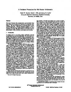
A SAT-based Decision Procedure for the Boolean Combination of Difference Constraints DTP: 35 variables on real domain

3

DTP: 35 variables on integer domain

3

10

171

10 TSAT++ MathSAT CSPi Tsat SEP

2

TSAT++ Epilits SEP 2

10

10

1

1

cpu time

10

cpu time

10

0

0

10

10

−1

−1

10

10

−2

10

−2

2

4

6

8 ratio

10

12

14

10

2

4

6

8 ratio

(a)

10

12

14

(b)

Fig. 1. Performances on (a) randomly generated DTPs, with 35 real valued variables (b) randomly generated DTPs, with 35 integer valued variables. Systems are stopped after 1000 seconds. (a),(b) back: satisfiability percentage. Real−life benchmarks

3

10

TSAT++ MathSAT SEP 2

ordered cpu time

10

1

10

0

10

−1

10

−2

10

0

5

10

15

20

25 benchmarks

30

35

40

45

50

Fig. 2. Performances on real-world problems. Systems are stopped after 1000 seconds.

the number n of arithmetic variables, a positive integer L such that all the constants are taken in [−L, L]. Then, (i) the number of clauses m is increased in order to range from satisfiable to unsatisfiable instances, (ii) for each tuple of values of the parameters, 100 instances are generated and then given to the solvers, and (iii) the median of the CPU time is plotted against the m/n ratio. The results for k = 2, L = 100 and n = 35 are given in Figure 1: Plots (a) and (b) show the performances when the variables are real and integer valued respectively. When m/n ≥ 6, TSAT++ clearly outperforms the other systems: In the peak region, the solver that is closer to TSAT++ in this domain, namely Epilitis, is a factor of 6 slower on 35 variables (cf. plot (b)). This is a very positive result, taking into account that Epilitis only works on DTP with k = 2, and it has been thoroughly tested and optimized on this type of problems (see [15]). All the other systems are about 2 orders of magnitude slower than TSAT++ in the peak region. TSAT++ has been run with early pruning and pre-processing enabled, and these are fundamental for its performances on this test set: Without early pruning or pre-processing, TSAT++ on the peak is slower of 2, 1 order of magnitude respectively. The fact that these two techniques are important comes at no surprise, and confirm previous results in [1]. The new look-ahead, heuristics and look-back mechanisms used by TSAT++ explain the 2 orders gap with respect to Tsat. Finally, we also considered problems with n = 30, 40, 45, 50: As the number of variables increases, the performance gap between TSAT++ and the other systems also increases.

172

Alessandro Armando et al.

5.3 Comparative evaluation on real world problems In this paragraph we consider 1. the 40 post-office benchmarks introduced in [2], coming in 4 series (consisting of 7, 9, 11, and 13 instances respectively) of increasing difficulty, and 2. the 16 hardware verification problems from [14], 9 (resp. 7) of which are with real (resp. integer) valued variables. The post-office benchmarks represent bounded model checking for timed automata; the hardware verification suite include scheduling, cache coherence protocol, load-store unit and out-of-order execution problems. By looking at the results of MathSAT, SEP and TSAT++ on the post-office problems, our first observation is that SEP is not competitive on these problems: On 13 of the hardest instances, SEP had a segmentation fault in 11 cases, and on the other 2 hardest instances SEP is outperformed by different orders of magnitude by TSAT++ and MathSAT. Our second observation is that TSAT++ (with pre-processing and assignment reduction) performs better than MathSAT, up to a factor of 6, on each single instance: This is particularly remarkable given that the authors have customized a version of MathSAT explicitly for this kind of problems. Considering the hardware verification problems, all of them are easy to solve (less than 3s) for all the three solvers, except for SEP that timeouts on one instance. Of the 9 (resp. 16) runs of MathSAT (resp. SEP and TSAT++), only 3 take more than 0.1s. These observations are confirmed by Figure 2, which gives the overall picture of the results for MathSAT, SEP and TSAT++ on the 49 instances with real valued variables: The x-axis is the number of instances solved by each solver within the CPU time specified on the y-axis.

D 50 50 100 100 250 250 500 500

S unique TSAT++ SEP SEP (no c.m.) MathSAT 4 N 0 0.03 0.12 0.05 4 Y 0.01 0.84 0.07 TIME 5 N 0.01 0.13 1.18 0.61 5 Y 0.04 10.20 0.17 TIME 5 N 0.08 0.95 52.20 5.4 5 Y 0.21 288.30 0.77 TIME 5 N 0.29 5.92 742.99 21.22 5 Y 1.05 TIME 4.85 TIME Table 1. Diamonds problems.

5.4 Comparative evaluation on hand-made problems Finally, we consider the “hand-made” diamonds problems from [14]. Given a parameter D, these problems are characterized by an exponentially large (2D ) number of Boolean models, some of which correspond to TRP-models; hard instances with a unique TRP-model can be generated. A second parameter, S, is used to make TRP-models larger, further increasing the difficulty. Variables range over the reals. Table 1 shows comparative results on the diamonds problems. The third column denotes whether the problem has a unique TRP-model; the remaining columns show CPU times for TSAT++ with reduction of assignment enabled, SEP with and without conjunction matrix and MathSAT.2 TSAT++ clearly performs best, often by orders of magnitude; instances with a unique solution are more difficult than non-unique ones, as expected, except for SEP without conjunction matrix. For this test set, of fundamental importance is the good interplay between TSAT++ look-back and consistency checking engines. In particular, the reduction of assignment step is fundamental: Without reduction, TSAT++ performances are significantly worse, up to the point that problems that are solved in 1 second, are not solved without reduction within the time limit. 2

The configurations employed were suggested by the authors of SEP and MathSAT.

A SAT-based Decision Procedure for the Boolean Combination of Difference Constraints

173

6 Conclusions In this paper we have presented TSAT++, an effective system for temporal reasoning that improves the stateof-the-art both on randomly generated, real world and hand-made problems. This is particularly remarkable given that some of TSAT++ competitors are optimized or even customized for solving specific classes of problems. The good performances exhibited by TSAT++are due to (i) the use of new techniques, some of which coming from the SAT literature, and (ii) their effective interplay.

References 1. A. Armando, C. Castellini and E. Giunchiglia. 1999. SAT-based procedures for temporal reasoning. In Lecture Notes in Computer Science, volume 1809, 97–108. 2. G. Audemard, P. Bertoli, A. Cimatti A. Kornilowicz and R. Sebastiani. 2002. A SAT based approach for solving formulas over boolean and linear mathematical propositions. In Proc. CADE. 3. R. J. Bayardo, Jr. and D. P. Miranker. 1996. A complexity analysis of space-bounded learning algorithms for the constraint satisfaction problem. In Proc. AAAI, 298–304. 4. T. H. Cormen, C. E. Leiserson and R. R. Rivest. 1998. Introduction to Algorithms. MIT Press. 5. R. Dechter, I. Meiri and J. Pearl. 1991. Temporal constraint networks. Artificial Intelligence 49(1-3):61–95. 6. A. Gerevini and M. Cristani. 1997. On finding a solution in temporal constraint satisfaction problems. In Proc. IJCAI. 7. E. Giunchiglia, M. Maratea and A. Tacchella. 2003. Look-ahead vs. look-back techniques in a modern SAT solver. Accepted to SAT. 8. D. Le Berre and L. Simon. 2003. The essentials of the SAT’03 competition. In Proc. SAT. LNCS 2919. 9. C. M .Li and Anbulagan. 1997. Heuristics based on unit propagation for satisfiability problems. In Proc. IJCAI. 10. M. W. Moskewicz, C. F. Madigan, Y. Zhao, L. Zhang and S. Malik. 2001. Chaff: Engineering an Efficient SAT Solver. In Proc DAC. 11. A. Oddi and A. Cesta. 2000. Incremental forward checking for the disjunctive temporal problem. In Proc. ECAI. 12. P. Prosser. 1993. Hybrid algorithms for the constraint satisfaction problem. Computational Intelligence 9(3):268– 299. 13. K. Stergiou and M. Koubarakis. 1998. Backtracking algorithms for disjunctions of temporal constraints. In Proc. AAAI. Also Artificial Intelligence 120(1):81–117. 14. O. Strichman, S. A. Seshia and R. E. Bryant. 2002. Deciding separation formulas with SAT. In Proc. CAV. LNCS. 15. I. Tsamardinos and M. Pollack,. 2003. Efficient solution techniques for disjunctive temporal reasoning problems. Artificial Intelligence, 151(1-2):43–89.