A Scheme for the Evolution of Feedforward Neural Networks using BNF-Grammar Driven Genetic Programming Athanasios Tsakonas and Georgios Dounias University of the Aegean, Dept. of Business Administration, 8 Michalon Str., 82100 Chios, Greece, Phone: +30-271-35165, Fax: +30-271-93464 e-mail:
[email protected],
[email protected]
ABSTRACT: This paper presents our attempt to automatically define feedforward neural networks using genetic programming. Neural networks have been recognized as powerful approximation and classification tools. On the other hand, the genetic programming has been used effectively for the production of intelligent systems, such as the neural networks. In order to reduce the search space and guide the search process we employ grammar restrictions to the genetic programming population individuals. To implement these restrictions, we selected to apply a context-free grammar, such as a BNF grammar. The proposed grammar extends developments of cellular encoding, inherits present advances and manages to express arbitrarily large and connected neural networks. Our implementation uses parameter passing by reference in order to emulate the parallel processing of neural networks into the genetic programming tree individuals. The system is tested in two real-world domains denoting its potential future use. KEYWORDS: genetic programming, context free grammars, cellular encoding, neural networks, thyroid, Pima Indians diabetes
INTRODUCTION Genetic Programming has been proved nowadays as a flexible methodology and a valuable tool in data mining [1]. The prime advantage of genetic programming over genetic algorithms, is the ability to construct functional trees of variable length. This property enables the search for very complex solutions. These candidate solutions, in standard genetic programming, are usually in the form of a mathematical formula. This approach is commonly known as symbolic regression process. Later paradigms extended this concept to calculate any boolean or programming expression. Thus, complex intelligent structures, such as fuzzy rule-based systems or decision trees have already been used as the desirable intention in genetic programming approaches [2,3,4,5]. The main qualification of this solving procedure is that the feature selection, and the system configuration, derive in the searching process and do not require any human involvement. Moreover, genetic programming, by inheriting the genetic algorithms' stochastic search properties, does not use local search -rather uses the hyperplane search-, and so avoids driving the solution to any local minimum. The potential gain of an automated feature selection and system configuration is obvious; no prior knowledge is required and, furthermore, not any human expertise is needed to construct an intelligent system. Nevertheless, the task of implementing complex intelligent structures into genetic programming functional sets in not rather straightforward. The function set that composes an intelligent system retains a specific hierarchy that must be traced in the GP tree permissible structures. This writing offers two advantages. First, the search process avoids candidate solutions that are meaningless or, at least, obscure. Second, the search space is reduced significantly among only valid solutions. Thus, a genotype - a point in the search space- corresponds always to a phenotype - a point in the solution space. This approach -known as legal searchspace handling method [6]- is applied in this work using a context-free grammar. Implementing constraints using a grammar can be the most natural way to express a family of allowable architectures. While each intelligent system -such as a fuzzy system- has a functional equivalent -by means of being composed by smaller, elementary functions-, what defines and distinguishes this system is its grammar. Although mapping decision trees or fuzzy rule-based systems to specific grammars can be relatively easily implemented, the execution of massively parallel processing intelligent systems -such as the neural networks- is not forthright. In order to explore variable sized solutions, usually a kind of indirect encoding is applied. The most common one is the cellular encoding [7] in which a genotype can be realized as a descriptive phenotype for the desired solution. More specifically, within such a function
set, there are elementary functions that modify the system architecture together with functions that calculate tuning variables. Current implementations include encoding for feedforward and Kohonen neural networks [7,14] and fuzzy Petri-nets [8]. In his original work, Gruau also used a context-free grammar - a BNF1 grammar- to encode indirectly the neural networks. On the other hand, in [8] a logic grammar - a context-sensitive one- is adapted to encode fuzzy Petrinets. In our work, we show that as long as the depth-first execution of the program nodes of a GP tree is ensured -which is the default-, a context-free grammar such as a BNF grammar is adequate for expressing neural networks. Gruau's original work has been faced some skepticism [9] on the ability to express arbitrarily connected networks. Later developments [10] seem to offer less restrictive grammar, though the cut function2 still maintained bounded effect. In our approach, we inherit present grammar advances proposed in [8] in his logic grammar for fuzzy Petri-nets and we suggest a BNF grammar for neural networks that is more descriptive than previous works. In the next section we present the design and the implementation of our system. The section that follows the design paragraph covers the results and our discussion in two real-world data sets: the Pima Indians diabetes data and the thyroid data. Finally, our conclusions are drawn in the last section as well as our suggestions for further research.
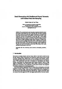
DESIGN AND IMPLEMENTATION In order to incorporate the architecture of feedforward neural networks into genetic programming one has to decide whether he will use direct or indirect encoding. Direct encoding, although it describes fixed sized neural networks effectively, in most problem cases is inefficient while the a-priori knowledge of the neural network's best architecture is not available. Thus, it seems normal to prefer a learning process that uses variable sized neural networks such as cellular encoding, a variation of indirect encoding. Our work is consisted of the application of a BNF grammar to encode indirectly variable length feedforward neural networks. The idea behind cellular encoding is that each individual program in the population is a specification for developing a neural network. As it can be seen from Figure 1, to implement neural networks we consider three types of places. First, input places, such as N1 and N2, associated with the system input values during run. Second, intermediate places, such as N3 and N4, and third, output places, such as N5 that represents the system outputs. The structure of a neural network for a particular problem must be restricted, in terms that if the problem requires a binary classification, then the network will have only two output places. The final output can follow the winner-takes-all concept -the output with the larger value is assumed as the system's output. Table I presents the manipulating functions. Manipulating functions initialize the inputs and/or insert additional places into the developing network. These functions are classified into two types, since there are two types of modifiable places, the input places and the intermediate places. N1
N3 N5
N2
N4
Figure 1. A simple feedforward neural network. Table I. Manipulating functions Name Description Input place sp1 Sequential division pp1 Parallel division in initialize the value Intermediate place sp2 Sequential division pp2 Parallel division stop Terminate the modification lnk Modify synapse (link) act Activate
Number of arguments 3 2 1 3 3 1 4 0
The implementation of a parallel processing system -such as neural networks- in a tree like the GP-tree that is executed depth-first, requires special handling of variables in order to emulate a breadth-first execution and simulate the parallel 1 2
BNF: Backus-Naur-Form for the definition of the cut function see the paragraphs that follow.
processing. Thus we selected to apply to all functions a parameter passing by reference for two variables: a parameter array Q and a parameter value V. The array Q keeps synapse values and the value V mostly handles activation results. In our implementation the parallel execution of each individual is ensured, by the proper handling of these variables. In order to avoid confusion, we should define explicitly the meaning of the arguments shown in Table I. These arguments correspond to the permissible children a parent GP-node may have in a GP tree. On the other hand, the array Q and the variable V, correspond to the internal implementation of the neural network's elementary functions into the GP tree and they enable variable sharing throughout an individual's execution, that is needed to simulate the parallel processing. In the following paragraphs, a short presentation is given for each of the functions together with an explanation of the implementation. Each function calls its arguments, passing the array Q and the variable V by reference, unless otherwise stated. For example, function pp2 creates copies of the (input) array Q before passing them to its arguments. • The sp1 function takes three arguments. The first and the third argument can be pp1 or sp1 (or in) functions. The second argument is a weight value. It calls sequentially the three arguments. Its application to the developing neural network is to add sequentially a node next to the node that is applied. • The pp1 function has two arguments. They can be pp1or sp1 (or in) functions. It feeds the arguments with copies of the array Q. It then saves the concatenation of them to array Q. It does not affect explicitly the variable V. Its modification to the developing neural network is to create a node in parallel to the node that is applied. • The in function has one argument. This argument is one of the network inputs. It initializes the array Q and the variable V to this value. • The sp2 function has three arguments. The first and the third argument can be pp2 or sp2 (or stop) functions. The second argument is a weight number. It calls sequentially the three arguments. Its application to the developing neural network is to add sequentially a node next to the node that is applied similar to sp1. • The pp2 function takes three arguments. The first and the third argument can be pp2 or sp2 (or stop) functions. The second argument can be a lnk or an act function. It feeds the three arguments with copies of the array Q. It then saves the concatenation of the first and the third argument to array Q. It does not affect explicitly the variable V. Its modification to the developing neural network is to create a node in parallel to the node that is applied, similar to pp1. • The stop function takes one argument. This argument is a bias number. It adds the bias number to the value V and performs hyperbolic tangent activation. The result is saved to variable V. The array Q is also initialized with the value V. • The lnk function takes four arguments. The first argument is a number that calculates the number of the synapse to be processed. The number derives by the application of the formula Z mod N, where Z is the number of existing synapses (kept in array Q) and N is the value of the argument. The second argument is a weight number and updates the weight of the selected synapse. The third argument is a cut number and cuts the selected synapse if and only if the cut value is 1 and the number of inputs to this place is greater than 1. The fourth argument can be again a lnk function or an act function. • The act function summarizes the elements (synapse inputs) in the array Q and returns the result to V. It takes no arguments. Table II. BNF grammar for the neural network. Symbol Rule
::= ::= < PROG> ::= ::=SP1 | PP1 | ::= ::=float in [-1,1] ::= SP2 | PP2 | ::= ::= | ::= float in [-1,1] ::=LNK ::=ACT ::=integer in [1,256] ::=integer in [0,1] ::=data attribute (system input)
As seen from the previous, there are additional functions that assist the selection of a number into a given range and a given precision. These functions are presented below.
The weight number function returns a float in the range [-1,1] with a precision of 0.00390625. The bias number function returns a float in the range [-1,1] with a precision of 0.000244140625. The cut number function returns an integer from the set {0,1}. The number function returns an integer in the range [1,256]. The selection of the precision for the weight number and the bias number is similar to the existing literature [10]. The BNF grammar production rules used for implementing the neural network are summarized in Table II. This example grammar corresponds to a binary decision neural network - with two independent outputs. A tree starts with the symbol. As it can be seen from the design of this grammar, there is no limit on how many cut functions could be applied in a node. This is an upgrade from previous implementations - where the number of effective cut functions was limited - and enables to a larger set of neural networks to be expressed within the search process.
RESULTS AND DISCUSSION The model is tested in two data sets from the medical domain. These data sets have been taken unmodified by a collection of real-world benchmark problems, the Proben1 [11] that has been established for neural networks. Table III shows the problem complexity of these data sets. Each data set is separated into a training set, a validation set and a test set. The training set is consisted of 50% of the data and the rest 50% is divided equally between the validation set and the test set. During the training phase, the validation set is used to avoid overfitting. For example, a solution which has better classification score in the training set, is adapted as new best solution if and only if the sum of classification scores of both training and validation sets is the same or better than the best solution's respective score. The genetic programming parameter settings are presented in Table IV. For comparison reasons, we selected to keep the same settings in both problems. Table III. Problem complexity for two real-world benchmarking data sets Inputs Problem Attributes continuous discrete diabetes 8 8 0 thyroid 21 6 15 Table IV. Genetic Programming Settings Parameter Population Size GP implementation Selection Maximum number of generations Crossover probability Mutation probability (overall) Shrink mutation probability (relative to overall) Node mutation probability (relative to overall) Number mutation probability (relative to overall) Maximum size of individual Function Set and Terminal Set Fitness function
Classes
Examples
2 3
768 7200
Setting 4000 individuals Steady-state grammar driven GP Tournament of 6 with elitist strategy 200 65% 35% 40% 30% 30% 650 nodes See Table I and Table II Sum of correct classifications
PIMA INDIANS DIABETES DATA The first data we apply the system is the Pima Indians diabetes data. It is a binary classification problem. The aim is to diagnose whether or not a patient has diabetes. The class probabilities are 65% and 35% for no diabetes and diabetes correspondingly. The attributes are presented in Table V. Although there are not missing values in this data, there are several senseless zero values that introduce some errors into the dataset. In [12], a linear genetic programming approach is applied, and for the same dataset -diabetes1- an average classification score of 76.04% is referred for the test set. In [11], this average classification score for the test set is 75.9% using neural networks trained with RProp [13]. The solution presented in Appendix, was achieved after 92,000 iterations (23 generations) and has accuracy 76.96% (147/191) in the test set. The accuracy in training and validation sets is 83.76% and 70.68% respectively. Although the results seem very promising, extended experimentation has to be completed in order to obtain average training results.
Table V. Diabetes attributes Name Attribute T1 Number of times pregnant T2 Plasma glucose concentration a 2 hours in an oral glucose tolerance test T3 Diastolic blood pressure (mm Hg) T4 Triceps skin fold thickness (mm) T5 2-Hour serum insulin (mu U/ml) T6 Body mass index (weight in kg/(height in m)2) T7 Diabetes pedigree function T8 Age (years) THYROID DATA The second data we selected to apply our model is the thyroid database. The aim is to diagnose overfunction, normal function, or underfunction of the thyroid. The class probabilities are 5.1%, 92.6% and 2.3% respectively; entropy is 0.45 bits per example. There are 21 attributes, 6 of them of continuous value and 15 of them of discrete (0 or 1) value. A good classifier has to have accuracy better than 92% [11]. The solution presented in Figure 2 was accomplished after 4,000 iterations (1 generation) and has accuracy on the test set 94.44% (1699/1799). The classification score in the training set and the validation set is 93.8% (3375/3598) and 93.71% (1686/1799) accordingly. As it can be observed, even very early results in the search process of this problem, may produce systems with satisfying accuracy. This result verifies that this data may be classified adequately by linear systems [11]. It is seen also, that a relatively small number of attributes (3 out of 21) are enough for obtaining such classification accuracy. The same dataset has been used as benchmarking set in literature. In [12], the average classification score, using linear genetic programming, reaches, for the test set, the 98.09%. In [11], a neural network application, using RProp, achieves 97.62% average accuracy on the test set. ANN PROG In V17 -0.601563 PROG SP1 In V2 -0.980469 Stop -0.993164 -0.824219 PROG In V21 -0.453125
-0.601563
V17 -0.993164 V2 V21
(a)
Out =# max(O1,O2,O3) -0.980469
-0.824219 -0.453125
(b)
Figure 2. Solution after first generation (4,000 iterations): (a) program individual, (b) network representation.
CONCLUSIONS AND FUTURE WORK In this work, we presented our approach to the evolutionary development of feedforward neural networks using genetic programming. While our intention was to enable arbitrarily large and arbitrarily connected neural networks, we selected to implement an indirect encoding variation for the neural networks, the cellular encoding. The latter is expressed, within this work, using a BNF grammar that considers current grammar advances found in literature. Our implementation makes use of parameter passing by reference among genetic programming functions, in order to simulate the parallel processing of neural networks. Two real-world datasets from the medical domain are used to test the system. These two databases were preferred since they are characterised by different type of complexity. The first set, the Pima Indians diabetes data, represents a binary classification task and is assumed to involve noise. The second set, the thyroid data, is a classification between three classes, it has a relatively large number or records and classification scores found in literature are high. Our first results for the Pima Indians diabetes data seem very promising and highly comparative to those found in literature. For the second data, the thyroid database, very early
results are considered good, though they are definitely less accurate than those found in literature. However, more experimentation has to be accomplished in both domains, in order to secure transparent results. Further research should be accomplished in the testing on different domains. A number of separate runs should be included for each data in order to attain average classification scores. Moreover, within the same data set testing, different subsets for the training, validation and test sets should be considered, in order to avoid any data selection bias. On the other hand, the system should be tested with various genetic programming parameter settings. A comparison with neural networks derived by context-sensitive grammars [14] could present valuable results. Finally, a comparison with other genetic programming-derived intelligent systems -such as fuzzy rule-based systems and decision trees- could offer a clear view on the efficiency of this approach among similar ones.
REFERENCES [1] Koza J.R., Bennett III F.H., Andre D., Keane M.A., "Genetic Programming III", Morgan Kaufmann Publ., Inc.,1999 [2] E.Alba, C.Cotta, J.M.Troya, "Evolutionary Design of Fuzzy Logic Controllers Using Strongly-Typed GP", In Proc. 1996 IEEE Int'l Symposium on Intelligent Control., pp. 127-132. New York, NY., 1996 [3] Koza J.R., "Genetic Programming: On the Programming of Computers by Means of Natural Selection", Cambridge, MA, MIT Press., 1992 [4] Tsakonas A., Dounias G., "Hierarchical Classification Trees Using Type-Constrained Genetic Programming", in Proc. of 1st Intl. IEEE Symposium in Intelligent Systems, Varna, 2002 [5] Tsakonas A., Dounias G., Axer H., von Keyserlingk D.G., "Data Classification using Fuzzy Rule-Based Systems represented as Genetic Programming Type-Constrained Trees", in Proc. of the UKCI-0, 2001, pp 162-168 [6] Yu T., Bentley P., "Methods to Evolve Legal Phenotypes". In Lecture Notes in Comp.Science 1498, Proc. of. Parallel Problem Solving from Nature V, 1998, pp 280-291 [7] Gruau F., "Neural Network Synthesis using Cellular Encoding and the Genetic Algorithm", Ph.D. Thesis, Ecole Normale Superieure de Lyon, anonymous ftp:lip.ens-lyon.fr (140.77.1.11) pub/Rapports/PhD PhD94-01-E.ps.Z [8] Wong M.L., "A flexible knowledge discovery system using genetic programming and logic grammars", Decision Support Systems, 31, 2001, pp 405-428 [9] Hussain T., "Cellular Encoding: Review and Critique", Technical Report, Queen's University, 1997, http://www.qucis.queensu.ca/home/hussain/web/1997_cellular_encoding_review.ps.gz [10] Gruau F., Whitley D., Pyeatt L., "A Comparison between Cellular Encoding and Direct Encoding for Genetic Neural Networks", in Koza J.R., Goldberg D.E., Fogel D.B., Riolo R.L. (eds.), Genetic Programming 1996: Proceedings of the First Annual Conf., pp 81-89, Cambridge, MA, 1996, MIT Press [11] Prechelt L., "Proben1 - A set of neural network benchmark problems and benchmarking rules", Tech.Rep. 21/94, Univ. Karlsruhe, Karlsruhe, Germany, 1994 [12] Brameier M., Banzhaf W., "A comparison of Linear Genetic Programming and Neural Networks in Medical Data Mining", in IEEE Trans. on Evol.Comp., vol.5,no.1, Feb 2001,pp 17-26 [13] Riedmiller M., Braun H., "A direct adaptive method for faster backpropagation learning: The RPROP algorithm", in Proc. IEEE Intl. Conf. Neural Networks, San Francisco, CA,1993,pp 586-591 [14] Hussain T., Browse R., “Attribute Grammars for Genetic Representations of Neural Networks and Syntactic Constraints of Genetic Programming”, in AIVIGI’98:, Workshop on Evol.Comp., Vancouver BC, 1998
APPENDIX (ANN (PROG (PP1 (In T8) (PP1 (In T3) (SP1 (PP1 (In T2) (PP1 (PP1 (PP1 (PP1 (In T6) (In T6)) (In T7)) (SP1 (PP1 (In T2) (PP1 (In T1) (PP1 (In T6) (PP1 (PP1 (In T6) (SP1 (PP1 (In T2) (PP1 (PP1 (In T6) (PP1 (PP1 (PP1 (PP1 (In T6) (In T6)) (In T7)) (SP1 (PP1 (In T2) (PP1 (In T1) (PP1 (In T6) (PP1 (SP1 (PP1 (In T2) (PP1 (In T2) (In T7))) -0.078125 (PP2 (PP2 (PP2 (Stop -0.976563) ACT (PP2 (Stop 0.972412) ACT (Stop -0.951660))) ACT (Stop -0.975830)) ACT (PP2 (Stop -0.992676) ACT (PP2 (Stop 0.972412) ACT (Stop -0.951660))))) (PP1 (In T1) (SP1 (In T8) -0.773438 (Stop -0.992676))))))) 0.078125 (PP2 (Stop -0.999756) ACT (Stop -0.999756)))) (PP1 (In T1) (SP1 (In T8) -0.773438 (Stop 0.992676))))) (In T7))) -0.078125 (PP2 (Stop -0.975830) ACT (Stop -0.976563)))) (PP1 (In T1) (SP1 (PP1 (In T6) (PP1 (In T3) (SP1 (PP1 (PP1 (In T1) (PP1 (In T6) (PP1 (SP1 (PP1 (In T2) (PP1 (PP1 (In T2) (PP1 (In T2) (PP1 (In T8) (PP1 (SP1 (PP1 (In T2) (PP1 (In T1) (PP1 (In T6) (PP1 (SP1 (PP1 (In T2) (PP1 (PP1 (In T1) (In T8)) (In T7))) -0.078125 (PP2 (PP2 (PP2 (Stop -0.976563) ACT (PP2 (Stop 0.972412) ACT (Stop -0.951660))) ACT (Stop -0.975830)) ACT (Stop -0.951660))) (SP1 (PP1 (In T2) (PP1 (In T2) (In T7))) -0.078125 (PP2 (Stop -0.975830) ACT (Stop -0.951660))))))) -0.078125 (PP2 (Stop 0.992676) ACT (Stop -0.992676))) (PP1 (In T1) (SP1 (In T7) -0.773438 (Stop -0.992676))))))) (In T7))) -0.078125 (PP2 (Stop -0.976563) ACT (PP2 (Stop -0.972412) ACT (Stop -0.958252)))) (PP1 (In T1) (SP1 (In T8) -0.773438 (Stop -0.992676)))))) (PP1 (PP1 (PP1 (PP1 (In T6) (In T6)) (SP1 (PP1 (In T2) (PP1 (In T2) (In T7))) -0.078125 (PP2 (PP2 (PP2 (PP2 (Stop -0.972412) ACT (Stop -0.951660)) ACT (PP2 (Stop -0.972412) ACT (Stop -0.951660))) ACT (Stop -0.975830)) ACT (Stop -0.958252)))) (SP1 (PP1 (In T2) (PP1 (In T1) (PP1 (In T6) (PP1 (SP1 (PP1 (In T2) (PP1 (In T1) (PP1 (In T6) (PP1 (SP1 (PP1 (In T2) (PP1 (In T2) (In T7))) -0.078125 (PP2 (Stop -0.975830) ACT (Stop -0.951660))) (PP1 (In T1) (SP1 (In T8) -0.773438 (Stop -0.992676))))))) -0.078125 (PP2 (Stop -0.992676) ACT (Stop -0.992676))) (PP1 (In T1) (SP1 (In T7) -0.773438 (Stop -0.992676))))))) -0.078125 (PP2 (Stop -0.999756) ACT (PP2 (Stop -0.999756) ACT (Stop -0.999023))))) (In T5))) -0.078125 (PP2 (Stop -0.999756) ACT (Stop 0.992676))))) -0.773438 (Stop -0.992676))))))) -0.078125 (PP2 (Stop -0.999756) ACT (Stop 0.999023)))) (In T7))) -0.078125 (PP2 (Stop -0.951660) ACT (Stop -0.992676))))) -0.019531) (PROG (PP1 (SP1 (PP1 (In T3) (In T6)) -0.859375 (PP2 (Stop -0.972412) ACT (Stop -0.951660))) (In T3)) 0.625000))
Figure 3. Neural network description for the diabetes data.