A Semantic Query Processing Strategy for the ... - Infoscience - EPFL

Cherry Picking: A Semantic Query Processing Strategy for the Evaluation of Expensive Predicates Fabio Porto1 , Eduardo Sany Laber2 ? , and Patrick Valduriez3 1

2

Ecole Polytechnique Federale de Lausanne (EPFL), LBD, Switzerland [email protected] PUC-Rio, Department of Informatics , Brazil [email protected] 3 INRIA and LINA, Nantes, France [email protected]

Abstract. A common requirement of many scientific applications is the ability to process queries involving expensive predicates corresponding to user programs. Optimizing such queries is hard because static cost predictions and statistical estimates are not applicable. In this paper, we propose a novel approach, called Cherry Picking (CP), based on the modelling of data dependencies among expensive predicate input values as a k-partite graph. We show how CP can be easily integrated into a cost-based query processor. We propose a CP Greedy algorithm that processes the graph by selecting candidate values that minimize query execution cost, and the Epredicate algorithm that processes tuples in pipeline following the CP approach. Based on performance simulation, we show that these algorithms yields executions up to 86% faster than statically chosen pipeline strategies.

1

Introduction

In several scientific applications a common requirement is the ability to process data objects, which can be very large, by scientific user programs, which can be very long running. For instance, some objects could be satellite images and some user programs could perform image analysis and take a long time to complete. In a database environment, execution of these user programs can be simply modelled as expensive user-defined predicates [1] which can be included in SQLlike queries. In traditional query processing, predicates are processed as early as possible. When predicates are expensive, this approach may be quite inefficient since it may lead to multiple user program invocations. As an example of an application with expensive predicates, consider the query in Example 1 that identifies regions with a given correlation among their pollution indexes and humidity factors. The input to the query has two data sources: the relational views Meteo(region,map) and Pollution (region, city, pollindexes), ?

Partially supported by FAPERJ (Proc. E-26/150.715/2003) and by CNPQ, through Edital Universal 01/2002 (Proc. 476817/2003-0)

where Meteo models meteorological images per region and Pollution stores pollution indexes for cities. Two scientific programs compute, respectively, a satellite image-based humidity factor and a pollution index from an array of collected pollution samples: Humidity(blob) : f loat and P ollutionInd(blob) : f loat. The scientific programs are registered in the database system as user defined functions [2] together with estimates of their per tuple execution cost (in seconds) and selectivity factor, as in [1]. Example 1. Select m.region,po.city From Meteo m, Pollution po Where m.region=po.region and Humidity(m.map) < 1.5 and PollutionInd(po.pollindexes) > 0.6

1.1

Processing of Expensive Predicates

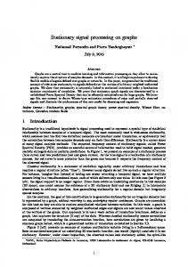
Let us discuss how this query can be executed. Let us assume that the average time for each invocation of the Humidity and Pollution programs are 3 and 1.5 minutes, respectively. A sequential query evaluation strategy that considers a Meteo relation with 10 distinct maps and a PollutionInd relation with 20 distinct pollution samples could take up to 3 × 10 + 1.5 × 20 = 60 minutes to be concluded. In such a scenario, an efficient QEP would place expensive predicates on the results of Humidity (H) and PollutionInd (P) user programs after the join operation, in the hope that the latter would eliminate some tuples and, as a result, reducing the number of program invocations. Let us now consider the ordering of expensive predicates. Assuming that some input values to predicates evaluate to false, different orders of evaluation produce unequal response times. Unfortunately, a static order is unable to adapt itself to fluctuations on data characteristics [3]. While such variations might be overlooked by traditional queries, their effect over the execution of expensive predicates is dramatic. As an example, consider the relation instance R in Figure 1 representing the join result between Meteo and Pollution 4 . Let us also assume that the expensive predicates evaluations over the input values return the following results: Reg1 → false, Reg2 → true, Reg3→ true, City1 → true, City2 → true, City3 → true, City4 → false. The most efficient evaluation would process tuples 1 to 3 by H(map) predicate and then process tuples 4 and 5 by expensive predicate P(pollindexes). Considering that we do not repeatedly process duplicate values [4], the elapsed-time for this query would be 4.5 minutes. 4

The values of map and pollindexes were replaced by Regi and Cityj for illustration purposes.

Map PollIndexes Reg1 City1

A1

A2

Reg1

City1

Reg2

City2

Reg3

City3

Reg1 City2 Reg1 City3 Reg2 City4 Reg3 City4

City4 a)

b)

Fig. 1. Input relation and its bipartite graph

On the other hand, a static order based strategy which processes H and then P would spend 10.5 minutes while the one which process P and then H would spend 9.0 minutes. Thus a natural question is why static order based strategies may perform so poorly. We believe that efficient query execution algorithms that involve expensive predicates must take into account the data-dependency induced by the input relation. This is the key idea behind the CP approach proposed in this paper.

1.2

Contributions

This paper makes three major contributions. First, we present the CP approach for processing expensive predicates based on the knowledge extracted from the associations among predicate input values. Such associations are modelled through a k-partite hypergraph (KHG). Second, we provide a cost based heuristic for integrating a CP algorithm into a query execution plan with expensive predicates. Finally, we propose two algorithms: a greedy algorithm that selects and processes the vertexes in the hypergraph following a greedy criteria and the Epredicate algorithm that selects values to be processed based on the CP approach but without requiring building the hypergraph. Our experiments demonstrate that for some very common scenarios, the greedy algorithm outperforms a static strategy by 86% on the average. The rest of this paper is organized as follows. Section 2 presents the CP approach in more details. Section 3 shows how the CP approach can be integrated into a query processor. Then, in Section 4.1, we present a KHG based CP approach algorithm using a greedy strategy. Next, in Section 4.2, a CP pipeline based approach is presented that evaluates the input relation to a set of expensive predicates without requiring the construction of a hypergraph. In Section 5, we evaluate the performance of the CP approach against static strategies. Section 6 discusses related work. Finally, Section 7 concludes.

2

The Cherry Picking (CP) Approach

We define the CP approach as the set of techniques and algorithms that take advantage of the data-dependency among input attribute values in order to evaluate a query with expensive predicates. The approach name, Cherry Picking, stands from its main principle of guiding the processing of expensive predicates towards the selection of best values within the whole set of input that minimize query execution time, similar to what one would do when picking cherries in a cherry tree. In this Section, we formally introduce the CP approach. We begin by specifying the type of queries we focus on this paper. Next, we show how to build the KHG from expensive predicates input values. We illustrate the process with the query in Example 1. Having presented the KHG, we are able to formalize our optimization problem for which the CP-algorithms are employed. 2.1

Preliminaries

In this paper, we focus on the evaluation of conjunctive SPJ (select, project, join) queries with both simple and expensive predicates. A predicate is expensive if it evaluates on the result of a user program that was registered in the database system as expensive. In this paper, we concentrate on programs of the user-defined simple function (UDSF) type, that take a tuple as input and produce a scalar value as output. For the sake of presentation, we assume that functions receive only one attribute as input. A consequence of focusing on UDSF functions is that we restrict the discussions in this paper to unary expensive predicates, i.e. we do not treat expensive joins. We consider a query execution plan (QEP) structured as an operator tree where internal nodes are operators and leaf nodes are input relations. Different shapes of trees can be considered: left-deep, right-deep or bushy. In this paper we make no restrictions regarding the shape of the operator tree. A QEP is defined as P = {ρ, Ω, ≺}, where ρ is a set of relations, Ω is a set of operators that includes: algebraic operators, control operators and modules (see brief presentation bellow) and ≺ is a set of ordering operators whose elements define an execution order between operators in Ω (which we will read as preceds in execution order). We say that ωi ≺1 ωj iff executing ωi produces a result that is consumed by ωj . We also say that one operation ωi immediately precedes () another operation ωj in Ω, if ωi ≺1 ωj and not ∃ ωk ∈ Ω, such that ωk ≺1 ωj and ωi ≺1 ωk . 0 0 0 0 We further define a QEP fragment P = {ρ , Ω , ≺}, with P ⊆ P , if, forall 0 0 ωi , ωj ∈ Ω , ωi 6= ωj , either ωi ≺1 ωj or ωj ≺1 ωi in P . 0 A QEP fragment P is said to be a set of expensive predicates (SEP) if all 0 operators in Ω are expensive predicates. In addition, we use the term input relation to a SEP S in a QEP P to denote the relation produced by an operation ωi , with ωi ∈ Ω and ωi ∈ / S, and ∃ ω j ∈ S | ω i  ωj .

As a last definition regarding a QEP, we denominate a Module, a QEP fragment implementing a specific execution semantic. Finally, a hypergraph G = (V, E) is a mathematical structure, where V = {v1 , . . . , vn } is the set of vertexes and E = {e1 , . . . , em } is the set of hyperedges. A hyperedge e ∈ E is a subset of V . We define the degree d of a vertex vi as the number of hyperedges containing vi . Two vertexes, u and v, are adjacent if there is an hyperedge e such that u ∈ e and v ∈ e. A hypergraph G is k−partite if V can be partitioned into k disjoint subsets A1 , A2 , . . . , Ak such that |e ∩ Ai | ≤ 1, ∀ e ∈ E, i = 1, . . . , k. 2.2

Modelling the Input Relation through a k-partite Hypergraph

The CP approach promotes the efficient execution of a set of k expensive predicates in a query β by capturing the data dependency among expensive predicates input values through a k-partite hypergraph (KHG). A KHG is an abstract representation of the input relation (see Figure 1 a) e b)). Each partition of the hypergraph corresponds to input values to an expensive predicate in the SEP. Vertexes in a partition represent distinct values in an input relation attribute bound to the associated expensive predicate. Thus, each hyperedge in the KHG is taken from the input relation tuple. Given an hyperedge e ∈ E, corresponding to a tuple in R, we say that e is true if the evaluation of the set of expensive predicates on its vertexes values returns true. Otherwise, we say that e is false. As an example, consider the input relation R(map, pollindexes), as in Figure 1. R attributes are bound to the set of expensive predicates SEP = {Humidity, P ollutionInd}. The corresponding KHG, is defined as G = {A1 ∪ A2 , E}, where the partitions A1 and A2 contain distinct URIs for the values in attributes map and pollindexes, and the edges in E correspond to tuples in R. Then, A1 = {Reg1, Reg2, Reg3}, A2 = {City1, City2, City3, City4} and E = {(Reg1, City1), (Reg1, City2), (Reg1, City3), (Reg2, City4), (Reg3, City4)}. In this context, the bipartite (2-partite) graph G is equivalent to the R input relation regarding the evaluation of the expensive predicates. In order to produce a valid tuple from query β, the evaluation of vertexes values in the corresponding edge in G must be true for all expensive predicates in β. On the other hand, whenever the evaluation of a vertex value returns false, all the edges which contain that vertex, and their respective tuples, are eliminated. 2.3

Problem Formulation

Thus, given a query β with a set of expensive predicates, we want to devise a cost-based heuristic model to evaluate the adequacy of assigning a CP module for processing a SEP. Also, given an input relation to the SEP, we want to devise a CP algorithm that determines, as fast as possible, whether each tuple is true or false. Finally, we want to integrate the CP approach into a QEP.

3

Integrating CP into Query Processors

In this Section, we discuss the integration of the CP approach into modern query processors. Query processing consists of two main phases 5 : query optimization and execution. During query optimization, an optimal QEP is produced based on the analysis of statistics collected from query objects and a cost model. Next, the QEP is submitted to a query execution engine that executes the operations in the QEP accordingly. 3.1

An Optimization Strategy for the CP Approach

The integration of the CP approach into query processing also consists of two phases. During the optimization phase, a query execution plan is created following the traditional dynamic programming strategy for plan enumeration [5] adapted to the placement of expensive predicates according to a rank order [1]. In this strategy, each predicate δi is annotated with a rank computed 1−sel(δi ) . as:rank(δi ) = pertuplecost(δ i) Once the QEP has been produced, we exercise one extra pass through it to analyze the adequacy of adopting the CP approach. The process traverses the QEP bottom-up looking for sets of expensive predicates. When a SEP is found, a cost-based heuristic (see equation (1)) evaluates the benefit of assigning a CP module to process it. Different cost models may be distinguished according to the specifics of an application. We opted for a conservative heuristic, which assigns a CP module to a QEP fragment with a SEP whenever the former estimated overhead cost represents a fraction of the registered per tuple invocation cost of the least expensive predicate in the SEP. More formally, the CP-module is employed if overhead(CP module) ≤ ρ ∗ δi .pertuplecost(),

(1)

where overhead(CP module) models the extra cost incurred when adopting the CP approach (see Section 4.1 for a concrete example), δi .pertuplecost() is the per tuple cost of the least expensive predicate in the analyzed SEP and ρ is a constant 6 . The left side of equation (1) should be adapted to the type of CP algorithm chosen for evaluating a SEP. In addition, the ρ constant provides for a tuning mechanism to be modified according to application characteristics. If the CP approach overhead is considered negligible compared to the cost of the expensive predicates evaluation, then the QEP fragment is replaced by a CP module. A CP module implements the CP approach into a QEP. Its execution model follows the iterator interface (open(), getnext() and close()), which provides for a transparent integration into a QEP. Different CP modules can be designed according to the strategy adopted for implementing the CP approach. 5 6

Parsing and preprocessing have been left out for simplicity. we expect to predict an ρ value according to statistics on executions history

Once the traversal of the QEP is done, the second phase of query processing initiates where the new QEP is sent to the query engine for processing.

4

A CP Algorithm

In this Section, we give a general introduction to the class of CP algorithms and present two algorithms that implement it. We define a CP algorithm as a strategy for the selection of input attribute values in the input relation to be evaluated by a corresponding set of expensive predicates that minimizes the query elapsed-time. In [6], it was demonstrated that any CP algorithm will process, at least, a cover of the KHG , that is, a set C ⊂ V such that C ∩ e 6= ∅ for every e ∈ E. That is because at least one vertex from each hyperedge must be evaluated in order to decide whether such an hyperedge is true or not. In this paper, we initially propose a CP algorithm based on the KHG approach that implements a greedy strategy for computing a minimum cost cover for a KHG. Next, we present the Epredicate algorithm, which is a pipeline based strategy alternative for implementing the CP approach. 4.1

A KHG Greedy Algorithm

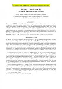
The greed algorithm selects the vertexes to be evaluated according to their degree in the KHG and associated expensive predicate’s rank. We name this index the vertex fanout and compute it as: F (ai,j ) = dai,j ∗rank(δi ), where ai,j corresponds to the j vertex associated to i bound attribute, dai,j is the degree of the ai,j vertex and δi is the expensive predicate bounded to i input relation attribute. Figure 2 presents the pseudo-code for the Greedy algorithm. In Step 1, the fanout is computed for each vertex in hypergraph G. The Step 2 consists of a loop. First, the vertex with highest fanout is selected for processing. Let a i,j be this vertex. If a predicate evaluation over ai,j value returns false, then all the hyperedges in graph G containing ai,j and the corresponding tuples, are eliminated. On the other hand, if the evaluation returns true, then ai,j is removed from every hyperedge which contains it. At the end of the loop every hyperedge with no more vertexes is written to the output and eliminated from G. Finally, ai,j is removed from V and the fanout of every vertex in V adjacent to ai,j is recalculated. This process continues until there are no more hyperedges left in G. The greedy CP-algorithm can be implemented in different ways. An efficient implementation uses a priority queue data structure to store the vertexes of G. The priority queue is ordered by the vertexes fanouts. Each cell of the heap stores four fields: id , value, fanout and p, where id is the vertex identification, value is its associated value, fanout is its fanout and p is a pointer for a list that stores the hyperedges which contain this vertex. Furthermore, a vector V is used to store the hyperedges of the graph. The entry V [e] holds three fields: a flag indicating if e has been deleted or not, an integer indicating the number of vertexes contained in e and a pointer for a list of vertexes in e. In addition, the vector index is used as

Greedy(G, β, δ1 , δ2 , · · · , δk ) Step 1: Compute F (v), for every v ∈ V Step 2: While (there are edges in E) ai,j ← argmaxv∈V {F (v)} N ← set of vertexes adjacent to ai,j at the current graph If δi (ai,j ) = 0 then Remove from E every hyperedge which contains ai,j . else Remove ai,j from every hyperedge e which contains it For every e ∈ E, with e = ∅ Output e; E = E − {e}; Remove ai,j from V Recompute F (v), for every v ∈ N Fig. 2. Pseudo code for the greedy CP algorithm

the tuple-id for the associated tuple. It is possible to show that this data structure allows for an O(mk log mk) time implementation of greedy CP-algorithm with small hidden constants, where m is the estimated cardinality of the input relation and k is the number of expensive predicates in the QEP fragment. Assuming the usage of the data structure described so far, the overhead cost for the greedy CP algorithm is computed as overhead(CP module) = c ∗ mk ∗ logmk, where c represents the average cost for one comparison operation. 4.2

A Pipeline Algorithm

A clear drawback of the KHG based CP approach is that it requires building the hypergraph in order to compute vertex degrees. As a result of this, it is a blocking strategy in respect to the data flow through QEP operators , which means that the whole input relation has to be consumed by the CP module before the first tuple can be evaluated by a CP algorithm. In this section we present a polynomial pipeline algorithm called Epredicate, that is based on the CP approach, but does not require building the hypergraph. Actually tuples are evaluated as soon as they reach Epredicate CP module. Epredicate considers estimates for the unitary cost of each attribute value evaluation. Its objective is to minimize the cost incurred during the evaluation of the input relation to a set of expensive predicates, by (1) maximizing the evaluation of least costly neighbors of each attribute value, and (2) subjected to the estimated cost of each attribute value. In other to illustrate Epredicate strategy, consider again the relation instance R in Fig.1 expressed as triples (attribute value, cost, result), where attribute value is the attribute value id; cost is the estimated attribute value evaluation cost and result is the result of evaluating an expensive predicate on this attribute value. Considering only distinct attribute values, the relation instance R

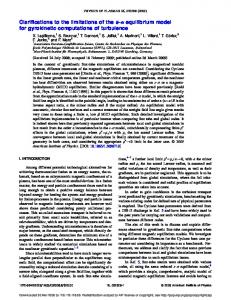
can be represented as: Map= {(Reg1, 2, f alse), (Reg2, 4, true), (Reg3, 3, true)}, PollIndexes= {(City1, 1, f alse), (City2, 2, true), (City3, 2, true), (City4, 1, f alse), (City4, 1, f alse)}. In Epredicate, each tuple is evaluated in non decreasing relative attribute value cost (RAVC) order. Thus, in the running example, the first tuple includes (Reg1,City1). According to (1), the least costly attribute value (City1, 1) is chosen for evaluation. In order to cope with (2), the relative cost of Reg1 is decremented by the cost of its evaluated neighbor (i.e. City1). Thus, now Reg1 RAVC is 1. As P (City1) = f alse, the tuple is discarded and a new one is read. It turns out that Reg1 now has a minimum RAVC, Reg1 = 1 and City2 = 2, so it is scheduled for execution. The result of H(Reg1) evaluation is false and the second tuple is eliminated. The third tuple is evaluated false, once H(Reg1) = f alse, and the fourth tuple is read. The least costly attribute value City4 is then scheduled for evaluation and returns false, which ends the execution. The final overall cost obtained by Epredicate in this example was 4, against a minimum cost of 3. Let k be the number of Expensive predicates. It has been shown that, for any given input, Epredicate yields an execution that is at most k times the cost of the set of attributes with minimum cost that one must read in order to decide which tuples match the query [7]. The epredicate algorithm is presented next: Epredicate(R(a1 , a2 , · · · , ak ), δ1 , δ2 , · · · , δk ) While (there are tuples in R) ti , o ← getnext tuple in R While (ti is not decided and ti is not ∅) vi ← RAV C(ti ) let ai,j |ai,j ∈ ti and min RAVC (vi,j ) ti ← ti − {ai,j } If δj (ai,j ) = 0 then ti is decided endIf Update RAVC for all ai,j in ti endWhile If ti = ∅ Output o; endIf endWhile Fig. 3. Pseudo code for the Epredicate algorithm

The main insight behind Epredicate algorithm is that to decide a tuple, at least one of its attribute values must be evaluated 7 . Thus, by considering a non decreasing cost order of evaluation for each tuple attribute value, a local 7

Which corresponds to a KHG vertex cover.

optimal solution is achieved. Nevertheless, in order to obtain a global solution, Epredicate adheres to the CP approach by taking into account the relative cost for each attribute value. This means that, a higher cost attribute value achieves its execution point when the sum of the costs of its less costly neighbors, in all tuple so far evaluated, equals to its estimated cost. Epredicate may use a data structure similar to that of the CP approach, once it needs to store attribute values relative costs until they get evaluated. Its overhead can be computed as overhead(Epredicate)= c ∗ m ∗ logk. Nevertheless, it allows to evaluate a query with expensive predicates in pipeline, in complete syntony with modern query processing techniques.

5

Validation

In this Section, we report on experimental results obtained by evaluating queries with expensive predicates using the CP approach. The experiments compare results from the greedy and the Epredicate CP algorithms with pipelined strategies [1]. We simulated both strategies and execute them over synthetically generated data. 5.1

Experimental Setup

The experiments were executed on a single 2.0GHz processor Dell machine running Linux kernel version-2.4.18-2, with 532MB of RAM. The simulation program employed GCC v. 3.1 and the data generator is a java program using jdk1.3.1. We consider one input relation R with 2 attributes, each bound to one expensive predicate. The data generator builds relations with randomly distributed values according to the parameters in Table 1. Values in each column are independently generated. Initially, for each column, we fill distAi slots, of a total of card slots, with a value between 1 and distAi , randomly selected using java Math.random method, normalized for the range of valid tuple numbers. Next, we fill each of the remaining slots with a randomly selected value between 1 and distAi . For each attribute, an extra column indicates the result of evaluating its corresponding expensive predicates over each of its values. The assignment of true values are randomly distributed along the tuples according to the specified selectivity factor of the correlated expensive predicate. The simulation consists of: picking a tuple for processing by an expensive predicate, adding to a counter a value corresponding to its estimated unitary cost and checking its evaluation column value for the result. False evaluations induce the elimination of the corresponding tuples, whereas true evaluations either keep the tuple for further predicate evaluations or send the corresponding tuples to the output. The simulation also imposes, during pipeline processing, that duplicate values are not considered, as if a caching mechanism prevented unnecessary program invocations.

Table 1. Parameters for simulation runs Parameter Meaning Values card Number of tuples 100-100.000 k Number of expensive predicates 2 distAi Number of distinct values in column R[Ai ] 1-100.000 costPi Unitary invocation cost of an user program Pi 1-10 selδi selectivity of expensive predicate δi 0.01-1

A run gives the results obtained for a given set of parameter values, as specified in Table 1. Each result value is obtained by averaging the results of 20 executions for the same set of parameters values. At each run, we register the vertexes evaluated by each expensive predicate and compute the query total cost for the CP and the pipeline strategies. 5.2

Performance Results

To obtain meaningful performance results, we ran three different experiments. Our experiments considered query Q1 in Example 2, where R(A,B) is an input relation to the expensive predicates s1 and s2 . Example 2. Select * From R Where s1 (A) and s2 (B) The first experiment analyzes the influence of the distribution of column distinct values on query execution. We considered a run with the following set of parameter values: S = {(card, 1000), (distA , 700), (sels1 , 0.3), (sels2 , 0.35), (costs1 , 3), (costs2 , 3)}. We registered 5 runs in which we varied the number of distinct input values on column B from 100 to 900, by steps of 100. Figure 4 a) shows the results of executing the CP greedy algorithm and two pipeline strategies: s1 s2 (s1 followed by s2 ) and s2 s1 (s2 followed by s1 ). We observe that, for 100 distinct values, CP outperforms s1 s2 by 86%, while it matches the results of s2 s1 . The important fact behind this experiment is that s1 s2 would be the choice of a rank order based strategy [1]. Thus, although a nice execution can be obtained from a pipeline strategy, it is not possible to predict it if only estimated cost and selectivity statistics are taken into account. As the number of distinct values grows towards 900, the pipeline lines in Figure 4 cross themselves, in a point near 700 distinct values, causing the s 1 s2 sequence to become the best choice for processing query Q1 . Note that statically computing the number of distinct values in columns of an intermediary relation, as the one produced by previous joins, can be very hard [8]. In addition, one can see the five runs as a single run on a relation of 5000 tuples where the distribution of distinct values varies for each 1000 tuples. In such a scenario,

no pipeline order can produce an efficient query execution. On the other hand, the CP approach adapts nicely to the fluctuations on distinct input values. In fact, it constantly produces the best evaluation order for predicates in query Q 1 . This is a direct consequence of considering the degree of each input value in the KHG, in addition to the predicate rank. Since most values in column A have no duplicates, a single evaluation of a vertex B, with average degree greater than 1 and selectivity 0.3, will very often eliminate multiple tuples, which saves s 1 from processing them.

3000

Total Cost

Total Cost

4000 2000 1000 0 CP s1s2 s2s1

5000 4000 3000 2000 1000 0

100 300 500 700 900 # distinct values to s2 a)

s2s1

selectivity of s2 b)

Fig. 4. CP versus pipeline

Our second experiment considers the impact of variations of the selectivity factor on query execution. We ran again query Q1 following the value set in S = {(card, 1000), (distA , 200), (distB , 900), (sels1 , 0.5), (costs1 , 6), (costs2 , 3)}. We computed 5 runs, in which the selectivity factor of predicate s2 varied from 10% to 90%, in steps of 10%. Here, we only compare the CP execution with the pipeline order s2 s1 , which should give the best rank order for all runs but the last. The rank value for predicate s1 is 0.083. If we consider an average degree of 4 for vertexes in A and of 1 for vertexes in B, we can conclude that only for very low selectivity factors the fanout of B vertexes would be prevalent over those of A vertexes. This analysis is confirmed in Figure 4 b). Only when the selectivity factor of s2 is 10% the rank order pipeline execution s2 s1 becomes close (24% above) to that of the CP approach. This is reasonable as long as s 2 is fast and very selective, which demonstrates the relevance of the number of distinct values over query execution performance. Even being selective and fast, s2 cannot be as effective as s1 as a result of a large difference between A and B in vertex degrees. When the selectivity factor of s2 has a maximum value of 90%, CP performs best in these runs, around 50% faster than s2 s1 . A further analysis of this experiment suggests the use of the CP approach for scenarios where selectivity factors are hard to predict. Under such hypotheses, estimating a 50% selectivity factor is a reasonable guess. The CP approach would compensate its lack of statistics with runtime knowledge of vertexes fanout yielding very good query execution performance (see Figure 4 b)). Our next experiment processes query Q1 over R where the fanouts of vertexes in A and B are symmetric with respect to half the number of tuples. We experi-

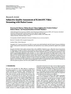
mented with a value set S = {(card, 1000), (distA , 450), (distB , 450), (sels1 , 0.5), (sel2 , 0.3), (costs1 , 6), (costs2 , 3)}. R tuples have an average of 50 distinct A values and 400 distinct B values from tuple 1 to 500. Then, the last 500 tuples show an opposite distribution of values. This is a case where no static order could lead to an optimal query execution time as the impact of an average vertex degree of 10 on estimated rank shifts the best choice for the first predicate to consume a tuple from one predicate to the other during R processing. The experimental results show that, in average, the CP outperforms the pipeline orders s2 s1 and s1 s2 by 65.4% and 63.3%, respectively. Finally, we report on first comparative results obtained for the Epredicate algorithm. This time we consider relation R(a, b, c) and the query: Select ∗ f rom R where s1 (a) and s2 (b) and s3 (c). As in the previous experiment, the relation instance R is generated from synthetic data and contains, in average, 100.000 tuples. We report on experiments regarding high selective expensive predicates, meaning that the selectivity factors of s1 , s2 and s3 are not greater than 0.25. Initial results can be found in Figure 5 that compares those obtained

Low selectivity

epredicate

5,000 4,000 3,000 2,000 1,000 0

greddy rank order

) 10 0, ,1

0,

,0 ,0 (0

,0 ,0 (0

)(1

)(1

1, (0

,0

,0

),(

0, (1 5) .2 (.2

5,

.2

5,

1,

1) 1,

1) 1,

,1 ,1 (1 5) .2 5, .2 5, (.2

1)

worst rank order

)

cost

8,000 7,000 6,000

Scenarios

Fig. 5. Results for:epredicate, greedy,pipeline

by running 5 different scenarios. The values in x axis correspond to the selectivity factor and unitary costs for expensive predicates s1 , s2 , s3 , in this order. As we can see, the greedy algorithm is almost always the best choice. It only looses, exactly to Epredicate, in the second scenario, by 0.8%, and presents its best result in the third scenario, showing a gain of up to 47% in respect to Epredicate. In the latter case, considering that all predicates present the same value for the selectivity factor and unitary costs, it was expected that the CP approach, which takes into account the correlation between values, would show better results than the others. Nonetheless, Epredicate demonstrates quite solid results beating best rank order in 4 out of 5 scenarios. Its worst result appears exactly when greedy shows its best outcome. This is mainly because Epredicate, as it is now, does not take into account the selectivity factor of expensive predicates.

6

Comparison with Related Work

The optimization of queries with expensive predicates has been the subject of extensive research [9, 1]. In some of these works, the traditional dynamic programming optimization strategy [5] is adapted to the evaluation of expensive predicates, i.e. predicates that range over the results of user programs. In particular, [1] proposes a predicate migration strategy, based on a polynomial time algorithm, in which predicates are ordered according to a rank value computed as a factor of their estimated selectivity factor and per tuple evaluation costs. [9] proposes the extension of the search space for potential QEPs by analyzing all possible orders of expensive predicates evaluation within each dynamic programming iteration, keeping the minimal cost QEP. In [10], user programs are modelled as relations allowing for techniques based on traditional query optimization strategies. These techniques, however, may yield sub-optimal execution times for queries such as in Example 1, for the following reasons. First, it is very difficult to predict the selectivity factors for the expensive predicates, as data do not really exist (they are generated by program evaluation). Even historical samples give very poor information about what may come in the future, considering that input data for published programs can come from very diverse data-sources within the Internet. Second, the query execution tree based on static predicate order is not sensitive to variations on distinct input value distributions applied to user programs. In this case, as shown in [11], physical operators implementing expensive predicates placed in the query tree higher nodes alternate between idleness periods, waiting for tuples to arrive from previous expensive predicates, with overload periods, with a queue of distinct input values that were paired with duplicate ones, in attributes bounded to previous expensive predicates 8 . In order to adapt to execution time conditions, some dynamic strategies have been proposed. [11] presents an strategy for evaluating expensive predicates in distributed queries. The strategy adaptively reacts to variances on estimated selectivity and cost of expensive predicates as well as on the effect of non-uniformity on data distribution. The query tree generated presents branches with expensive predicates in different pipeline orders. More recently, Madden and Hellerstein [3, 12] propose an interesting adaptive query execution framework, called Eddies. Rather than following a rigid QEP, in Eddies tuples are routed towards query operators following a flexible scheduling policy. A monitor module registers the consume/production rate of each operator. Whenever a synchronization point is detected, a lottery is ran between query operators. The most efficient query operator, according to the lottery policy, is scheduled for processing and is given the next tuple. The flexibility of Eddies allows for different plans to be evaluated during one single query execution. Although not specifically designed for dealing with expensive predicates, the strategy naturally fits expensive predicates within its adaptive operators schedule strategy. CP is an adaptive strategy in the way that 8

Caching [4] avoids processing programs over duplicate input values.

query execution conforms itself to a scheduling policy based on the relationship among expensive predicates input attribute values. As a matter of fact, one may use the CP approach as a scheduling policy for the Eddy framework for queries exclusively composed of unary predicates. The problem of applying Eddies to a distributed architecture has been studied in [13], where new tuple routing policies have been proposed. More recently, the adaptiveness promoted by Eddies, has been extended to deal with filtering on pipeline streams [14].

7

Conclusion

Optimizing queries involving expensive predicates corresponding to user programs has been hard because static cost predictions and statistical estimates are no longer useful. In this paper, we proposed a novel approach for the evaluation of expensive predicates in a query, called Cherry Picking (CP), based on the modeling of data dependencies among expensive predicate input values. This paper made three major contributions. First, we formally defined the CP approach for processing expensive predicates based on the knowledge extracted from the associations among predicate input values. Such associations are modeled through a k-partite hypergraph (KHG), where vertexes correspond to the predicates’ input values and edges correspond to tuples linking those values. Second, we proposed a cost based heuristic for integrating a CP algorithm into a query execution plan with expensive predicates. This makes it possible to integrate seamlessly the CP approach into modern query processors. We described the architecture of a CP module that fits in a query processor using the ubiquitous iterator model [15]. Finally, we proposed two algorithms that implement the CP approach. The greedy algorithm selects and processes vertexes in the hypergraph based on their fanout following a greedy criteria. The Epredicate distinguishes itself by providing a pipeline execution for the CP approach. Our experiments demonstrate that for some very common scenarios, the greedy algorithm outperforms a static pipelined strategy by 86% on the average. In addition, Epredicate’s initial results show that it is a very promising strategy for the CP approach, extending its applicability to a larger range of predicates. These experiments assumed accurate estimates for the static strategy which is impossible to achieve in practice. Furthermore, we did not count the overhead of managing statistics for the static strategy. Therefore, CP algorithms are much more efficient and simpler. In future work, we will extend the approach to dynamically react to variations on execution time conditions, like evaluation cost and selectivity factor. We will also extend it to deal with distributed data in the context of mediator systems. Finally, we plan to experiment with real data, which we will try to obtain from scientific applications.

References 1. Hellerstein, J.M.: Optimization techniques for queries with expensive methods. TODS 23 (1998) 113–157 2. Jaedicke, M., Mitschang, B.: User-defined table operators: Enhancing extensibility for ORDBMS. In: Proc. 25th Intl. Conf. on Very Large Data Bases, September 7-10, 1999, Edinburgh, Scotland, UK. (1999) 494–505 3. Avnur, R., Hellerstein, J.M.: Eddies: continuously adaptive query processing. In: Proc. of the 2000 ACM SIGMOD Intl. Conf. on Management of Data, May 16-18, 2000, Dallas, Texas, USA. (2000) 261–272 4. Hellerstein, J.M., Naughton, J.F.: Query execution techniques for caching expensive methods. In: Proc. 1996 ACM SIGMOD Intl. Conf. on Management of Data, June 4-6, 1996, Montreal, Quebec, Canada. (1996) 423–434 5. Selinger, P., Astrahan, M.M., Chamberlin, D.D., Lorie, R., Price, T.G.: Access path selection in a relational data base management system. In: Proc. Intl. Conf. on Management of Data, May 30 - June 1, 1979, Boston, Massachusetts,USA. (1979) 23–34 6. Laber, E., Porto, F., Valduriez, P., Guarino, R.: Cherry picking: A data dependency-driven strategy for the distributed evaluation of expensive predicates. In: Technical Report, PUC-Rio, Informatics Department, PUC-Rio.Inf.MCC01/02, 2002. (2002) 7. Laber, E.S., Carmo, R., Kohayakawa, Y.: Querying priced information in databases: the conjuntive case. In: Proc. of LATIN 2004,LNCS 2976, April 5-8, 2004, Buenos Aires, Argentina. (2004) 6–15 8. Ioannidis, Y.E., S.Christodoulakis: On the propagation of errors in size of join results. In: Proc. 1991 ACM SIGMOD Intl. Conf. on Management of Data, Denver, Colorado, May 29-31, 1991. (1991) 9. Chaudhuri, S., Shim, K.: Query optimization in the presence of foreign functions. In: Proc. 19th Intl. Conf. on Very Large Data Bases, August 24-27, 1993, Dublin, Ireland. (1993) 529–542 10. Chimenti, D., Gamboa, R., Krishnamurthy, R.: Towards on open architecture for LDL. In: Proc. 15th Intl. Conf. on Very Large Data Bases, August 22-25, 1989, Amsterdam, The Netherlands. (1989) 195–203 11. Bouganim, L., Fabret, F., Porto, F., Valduriez, P.: Processing queries with expensive functions and large objects in distributed mediator systems. In: Proc. 17th Intl. Conf. on Data Engineering, April 2-6, 2001, Heidelberg, Germany. (2001) 91–98 12. Madden, S., Shah, M., Hellerstein, J.M., Raman, V.: Constinuously adaptive continuos queries over streams. In: Proc. of 2000 ACM SIGMOD Intl. Conf. on Management of Data, June 4-6, 2002, Madison, Wisconsin, USA. (2002) 49–60 13. Tian, F., DeWitt, D.J.: Tuple routing strategies for distributed eddies. In: Proc. 29th Intl. Conf. on Very Large Data Bases, Sept 9-12, 2003, Berlin, Germany. (2003) 333–344 14. Babu, S., Motwani, R., Munagala, K., Nishizawa, I., Widom, J.: Adaptive ordering of pipelined stream filters. In: Proc. Intl. Conf. on Management of Data (SIGMOD), June 9-12, 2004, Paris, France. (2004) 15. Graefe, G.: Query evaluation techniques for large databases. ACM Computing Surveys 25 (1993) 73–170