The procedure calls for the generation and then thresholding of the gradient image, .... is considered to be the second most important center set, and so on.
440
IEEE TRANSACTIONS
ON CIRCUITS
AND
SYSTEMS,
VOL.
CAS-22,NO. 5, MAY 1975
A Spatial Clustering Procedure for Multi-Image Data ROBERT
M. HARALICK,
MEMBER,
IEEE, AND
Abstract-A spatial clustering procedure applicable to multi-spectral image data is discussed. The procedure takes into account the spatial distribution of the measurements as well as their distribution in measurement space. The procedure calls for the generation and then thresholding of the gradient image, cleaning the thresholded image, labeling the connected regions in the cleaned image, and clustering the labeled regions. An experiment was carried out on ERTS data in order to study the effect of the selection of the gradient image, the threshold, and the cleaning process. Three gradients, three gradient thresholds, and two cleaning parameters yielded 18 gradient-thresholds combinations. The combination that yielded connected homogeneous regions with the smallest variance was Robert’s gradient with distance 2, thresholded by its running mean, and a cleaning process that considered a resolution cell to be homogene&s if and only if at least 7 of its nearest neighbors were homogeneous. I. INTRODUCTION
C
LUSTER analysis has become in the last 30 years a multi-disciplinary technique of data analysis. Different methods of cluster analysis have been developed and applied in different areas of research. We will mention here only a few examples of the application of clustering in various disciplines (the order is of no significance). A clustering algorithm was used (Gose, [6]) as part of a procedure to identify breast cancer using radiographs and xerograms. A program that simulates the taxonomic process for plant classification (Rogei-s and Tanimoto, [19]) was applied to 300 herbarium specimens of manihot esculenta. Clustering techniques were applied to a collection of 1400 aeronautical documents in an information retrieval experiment (Sparck, [25]). Sneath proposed an analysis intended to produce taxonomic groups of bacteria. ISODATA clustering procedure (Wolf, [29]) has been used in a system for determining cloud motions. Cluster formation was used to diagnose 199 subjects in a psychiatric institute (Kaskey, [ 121). A hierarchical grouping technique was applied (Ward, [27]) to 25 test projiles based on art preference. Behavioral problems of deaf children (Haralick, [9]) were analyzed using clustering of variables. Different clustering techniques have been used to produce dendrograms for biological data (Sokal and Sneath, [24]). Dendrographs have also been used to represent mutual relationship among geologic variables (McCammon, [ 131). Clustering was used in image processing of remote sensing Manuscript received April 18, 1974; revised August 20, 1974. R. M. Haralick is with the Department of Electrical Engineering and IJ6J;;.rsity of Kansas Remote Sensing Laboratory, Lawrence, Kans. I. Dinstein was with the Deoartment of Electrical Engineering and University of Kansas Remote’Sensing Laboratory, Lawyence, Kans., as a Ph.D. candidate. He is now with the Communications Satellite Corporation, Clarksburg, Md.
ITS’HAK
DINSTEIN,
MEMBER,
IEEE
data (Haralick, [8], Smedes et al., [22]). This list does not intend to cover all the areas in which cluster analysis has been applied. It only illustrates the broad possibilities and the multidisciplinary nature of clustering. Clustering of any set of data is a subjective process that can be done in a number of different ways depending on the purpose of the classifier (Gilmour, [S]). For example, a zoologist might place a whale and a monkey in the same class whereas a fisherman will prefer the whale and tuna in the same class (Watanabe, [20]). There are some different objectives of cluster analysis. One objective is “. . . to gain more information about the structure of the data set” (Nagy, [14]). When dealing with large masses of data, cluster analysis might compress the data so that it can be analyzed more easily (Bonner, 1121). Such generalization might result in some loss of information but it may emphasize some other interesting parts qf the information as well as increase the efficiency with which large masses of data can be processed (Ward, [27]). Cluster analysis may “inform the researcher where the ‘action’ in his data set lies” (Haralick, [S]). It is a way of analyzing the details of the data’s structure (Ball, Cl]). Many clustering algorithms deal with measurements in ways that do not consider the order by which the measurements were taken. Indeed, for many problems, the order by which the measurements were taken or the spatial distribution of the units under consideration are irrelevant to the clustering process. In some cases, the relation between the order by which the data was collected and the clusters of the measurements depends very much upon the way the data was gathered. Such a case is in the clustering of image data. The resolution of the image data, when properly selected, should yield many measurements for each object of interest. Therefore, resolution cells of the same neighborhood are likely to belong to the same object, except at boundaries. We will refer to clustering procedures that take into account spatial relations between elements as spatial clustering procedures. Although image data is a good candidate for spatial clustering procedures, much of the clustering which has been done with multi-image data has not been spatial. This certainly is true for the measurement space iterative clustering techniques used on image data and described by Haralick [7], Darling and Juris (1970), Haralick and Dinstein [S], as well as the ISODATA or K-means clustering techniques used by Wacker and Landgrebe [26] and Smedes et al. [22] and many others in the remote sensing area. The artificial intelligence community has been an active user of spatial information from scene data. Much work
HARALICK
AND
DINSTEIN:
SPATIAL
CLUSTERING
PROCEDURE
441
the first step, points are assembled into row strips. This is based upon the assumption that “spatially adjacent vectors tend to belong to the same type of ground cover except at field boundaries.” Examining the resolution cells along the scan lines, similar resolution cells were assigned to strips. Each strip was terminated only when the addition of the next resolution cell would have increased the internal scatter of the strip above a given threshold. At that point, the formed strip was assigned to a cluster (or designated to start a new cluster), and the formation of a new strip began. The assignment of a strip to a cluster was done by comparing the strip to the cluster centers. The search for a cluster was done in a decreasing order of cluster populations, to save computation time and to eliminate a small group of abnormal components. The following is a formalization of this clustering proII. ON SOME SPATIAL CLUSTERING PROCEDURES FOR cedure. Let 1, Z, x Z,, and G be defined as before. Define MULTI-IMAGE DATA a function SS: Z, x Z, -+ S which partitions the spatial Let 2, = {1,2;. . ,N,} be a row index set and let Z, = domain Z, x Z, into a set S of spatially connected subsets, {1,2; *. ,N,} be a column index set. We call the set of s = {S,,S,; * *So}: The subsets Si, 1 I i I Q are the ordered pairs Z, x Z, the set .of resolution cells, or a “strips” that were mentioned previously. The spatial conspatial domain. Let Gi = { 1,2,. * . ,Ni} be a set of Ni grey nectivity of those strips is explained in the definition of the levels, and let G = G, x Gz x * * . x G, be the Cartesian function SS, which is given here in a sequential manner. product of the sets of grey levels G,,G,; 1*,G,. A digital 1) SS(l,l) = s,. multi-image is a function I: Z, x Z, --f G. The function, 2) SS(m,n) = Si if and only if SS(m, n - 1) = Si for I assigns a K-tuple of grey levels to every resolution cell in n & 1 or, SS(m - I, N,> = Si for n = 1, and Z, x Z,. Multispectral scanner data and multi-data aerial [Z(k,Z) - I(Si U {m,n})]2 I Ti image data take such a form. Using this notation, we now c (WE.%u t(m,n)l review three clustering procedures that take into account the spatial distribution of the grey level K-tuples. where N, is the last column in Z, x Z,, I(A) is the mean Haralick [7] introduced the following spatial clustering of the grey levels of the resolution cells belonging to A, and algorithm. Let S = (S,)? = 1 be a set of spatially con- T1 is a specified threshold. nected subsequences. of I. On each subsequence Si, define Let C = {C1,C2; 1*,C,} be a set of cluster codes. Define the empirically observed probability Pi(g) as the portion a function CC: S + C that assigns strips to clusters in the of resolution cells in Si which have K-tuple g. Define a following manner : function W: G + (0,l) by W, = maxi P,(g), i = I,. . *,Q. a) CC(S,) = C, ; W(g) is the highest relative frequency which the K-tuple g has in the subsequences Si, i = 1,2, * . *,Q. The range of the if d[W2M&)I I T2 b) CC(S,) = ;I’ function W consists of N, numbers, one for each K-tuple otherwise; and 2, of G. Define the sequence B = (gi 1gi E G) to be conif d [I(Sr),Z(Ci)] I T2 and Ci is the structed such that W(gi) r W(gj) for i I j. The elements ci, largest cluster for which it holds of the sequence B are ordered according to the respective C) CC(Sj) = c if the above condition does not descending order of their images through the function W. k, hold and C, is empty. The first element in the sequence B is that K-tuple which has a maximum observed probability Pi(gi) over all i = This clustering procedure was applied to multispectral 1,2;. . ,Q and all gi E G. The resolution cells containing that K-tuple (the first element in B) are considered to be data collected during the Imperial Valley study conducted the most important center set. The set of resolution cells in I by NASA in 1969. Flight lines of 5000 feet and 10 000 containing the K-tuple which is the second element in B feet by the University of Michigan aircraft were selected. is considered to be the second most important center set, This simple and economical clustering procedure was and so on. Once the collection of center sets is found, clusters demonstrated to be a feasible alternative to the conventional are “grown” around those centers. Two parameters govern terrain classification methods. Jayroe [I l] introduced a three-step spatial clustering the clustering process. One is the maximum number of procedure for multi-images. In the first step, a boundary expected clusters and the second is a probability cutoff parameter. map is prepared by thresholding of gradient images. The A spatial approach to imagery clustering was described two gradient images used are obtained by computing the by Nagy [IS]. Nagy’s clustering procedure is based on a Euclidian distance between nearest neighbors in the horisimple “chain algorithm” proposed by Bonner [2]. In zontal and vertical directions. In the second step, clusters
has gone into the definition of homogeneous regions and edge detection. Brice and Fennema [3] describe a procedure for partitioning an image into a large set of primitive regions each of which is typically a connected component having the same grey tone. Then a merging algorithm is applied to group together those regions of similar tone. Gradient and derivative computation algorithms have been used to find edges (Roberts, [17] ; Prewitt, [16] ; Hueckel, [IO]; Rosenfeld and Thurston, [21]). In this paper, we discuss extensions of these kinds of techniques to multi-image data sets. Such data sets occur naturally with multispectral scanners where the same scene is viewed in many wavelengths from the infrared through the ultraviolet as well as with aerial photography taken over the same area at different times.
442
IEEE TRANSACTIONS
are formed by scanning the boundary map with a fixedsize square of resolution cells. When the square hits a region in which there are no boundary cells, that region is assigned to cluster 1. The square is then moved farther, and if no boundary cells are encountered, the area within the square is assigned to cluster 1. The scanning continues until all possible cells are assigned to that cluster. Next, the square is moved until it hits a new region with no boundary cells, and the process repeats itself. In the third step, clusters are .merged according to their spectra measurements. Robertson et al. [ 181 describe a procedure for successively partitioning a multi-image into rectangular blocks. However, the final clustered images produced by the algorithm yield images which suffer from excessive blockiness.
ON CIRCUITS
AND
SYSTEMS,
MAY
1975
of resolution cells in Si, as seen by
BiE1 c GIW). #(si)W)ESi Before we define the cleaning operator, we define three types of neighborhoods as follows. Let N(i,j)
= {(m,n) E Z, x Z, [ m = i - 1 and In - j( I 1 or m = iandn
=j
- I>.
N(i,j) consists of the three nearest neighbors above (i,j) and the one to the left of (i,j). The Neighborhood
N(ij).
III. A SPATIAL CLUSTERING PROCEDURE BASED ON GRADIENT IMAGES
The spatial clustering procedure discussed here is based on Dinstein [4] and takes into account the distribution of the measurements in the measurement space as well as their distribution in the spatial domain of the. image. The procedure consists of 1) computation of a gradient image, 2) thresholding the gradient image, 3) cleaning the thresholded image, 4) labeling connected regions in the cleaned image, and 5) clustering the labeled connected regions. We now define functions and operators for those operations, using the notation as defined in the previous section. Define a function GZ: Z, x Z, + R to be the gradient image of I. GZ assigns a real number to each resolution cell in Z, x Z,. This real number is relative to the changes in grey levels of resolution cells in a neighborhood of that resolution cell. Therefore, we assume that when a resolution cell of the GI image contains a high number, it indicates that the resolution cell is close to a category boundary. It indicates that there is a significant change in the grey tones in its neighborhood. On the other hand, a low value assigned to a resolution cell in the GI image indicates that the resolution cell’s neighborhood is homogeneous. It indicates that all the measurement vectors assigned to the resolution cells in its neighborhood are close to its measurement vector. The objective of the proposed spatial clustering is to detect such homogeneous neighborhoods. The next step for achieving this objective is to threshold the GZ image in order to distinguish between homogeneous and nonhomogeneous areas. Define a function H : Z, x Z, + {LO} as follows: iff Gl(i,j) I 13 otherwise where 0 is a specified threshold. In our experiments, we have used a dynamic threshold defined as follows. Let Si = {(k,l) E Z, x Z, 1i - L < k I i + L} where L is a specified integer. The threshold 8i for the ith line of the gradient image is the mean of the gradient values
Let N*(i,j)
= {(m,n) E Z, x Z, I Im - il I 1 and In - jl I l}.
i-T-l-l t-y-q-y
The Neighborhood
N*(i,j).
I N*(i,j) Let A(i,j)
consists of the eight nearest neighbors of (i,j). = {(m,n) E Z, x Z, 1m < i or m = i and n < j}.
A(i,j) consists of all the resolution cells above and to the left of (i,j)
pi
TheNeighborhood
A(i, j) .
Define a cleaning operator (CL) by CL(i,j)
=
if #{(k,Z) E N*(i,j) otherwise
1H(k,l)
= l} L f12
where e2 is a specified threshold, and # denotes the number of elements in the set. The purpose of the cleaning operator is to eliminate fuzzy boundaries. We want the cleaned regions to be most representative of their clusters. Therefore, a resolution cell is considered as homogeneous if and only if at least 8 resolution cells in its nearest neighborhood are homogeneous. Now we define an operator which labels the connected homogeneous regions in the cleaned image. A region is said to be connected if and only if between any two of its resolution cells, there exists a sequence of resolution cells belonging to the region, such that each two consecutive cells in the sequence are nearest neighbors. This operator is similar to a labeling operator proposed by Rosenfeld [20]. Define the function C in a sequential manner, assigning the resolution cells line by line.
HARALICK
AND
DINSTEIN
: SPATIAL
CLUSTERING
443
PROCEDURE
1) If CL (1,l) = 0, set C(l,l) = 0. If CL (1,l) = 1, set C(1,l) = 1. 2) Suppose all the resolution cells in A(i,j) have been assigned, then a) if CL (i,j) = 0, set C(i,j) = 0, and b) if CL (i,j) = 1, then a. if {(m,n) E N(i,j) I C(m,n) # 0} # 4, set C(i,j) =
min(m,n)..(z.j) {C(m,n)I Ch4
Li = ((k,Z) 1CM(k,I)
C#Ljl.
2) CC&) = N if and only if d[l(L,),Z(N)] I e3 where I(&) is the mean of the grey level vectors of the resolution Cells in Lk, and I(N) is the mean of the grey level vector of resolution cells of regions that have been assigned to cluster N. d is a distance function defined on the set of grey level vectors, and 8, is a specified threshold. 3) Repeat Step 2 until no more assignments are possible. If all Lj, 1 I j I ,K were assigned, then stop. If not, then go to Step 4. 4) N= N+ 1. 5) CC(L,) = N if and only if’ max alli such that L, has not been assigned
3rd Bond
4th
Band
= i>.
Lr is the set of resolution cells belonging to the region labeled i. Let L = {L,,L2;- *,LK} be the set of all the regions labeled by the merging operator, and let CODE = {1,2; * *,K} of a set of cluster codes. Define a clustering function CC: L + CODE. The function CC assigns a cluster code to each one of the labeled connected and homogeneous regions. We define CC in a sequential manner, as follows. 1) N = 1. CC(LJ = N if and only if # Li =
#L, =
Band
Z 0, and
p. if {(m,n) E N(i,j) I C(m,n) # 0} - 4, set C(i,j) = 1 + maX(,d EA(i, j) Wv). The function C assigns labels to connected regions. These connected regions, however, are not maximal. Once connected homogeneous regions are detected and assigned integer labels, we want to detect regions which are maximal with respect to connectivity and homogeneity. This is done by merging all the homogeneous and connected areas which are connected to one another. We define a merging operator CM as follows. Let C, and C, be connected regions whose resolution cells were assigned by C. If there exists (i,j) E C, and (k,Z) E C, such that (i,j) and (k,Z) are nearest neighbors, CM merges those two regions by assigning min {(N,M)} to all the resolution cells of C, v C,. Apply the merging. The last operator to be defined is the clustering operator. The elements to be clustered are the labeled connected homogeneous regions. Let
maXlsjd
2nd
#L i*
6) Go to Step 2. The threshold 8, is specified by the. user as follows: Once the largest of the assigned regions is found, the distances between its mean and the means of the unassigned
Fig. 1. Four bands of the compressed ERTS image (Monterey Bay, July 25, 1972).
regions are computed, quantized, and displayed in a histogram. The user specifies the thresholds according to these histograms. IV. A PARAMETRIC STUDY The basic steps in the detection of connected homogeneous regions on an image are generation and then thresholding of the gradient image, cleaning of the thresholding image, and labeling the connected regions in the cleaned image. There are many ways of generating gradient images choosing the thresholding constant and cleaning the thresholded image. Because those are user selected factors, we have carried out an experiment in order to study the effect of some of these factors on the detection of connected homogeneous regions and the clustering of those regions. Three types of gradients, three thresholds for the gradient images, and two cleaning thresholds yielded 18 combinations of gradient-thresholds. A compressed strip (each resolution cell is the average of an 8 x 8 subimage on the original) of an ERTS image (Monterey Bay, ERTS Image identification 1002-18134, see Fig, 1) was processed using those 18 combinations. The average variance over the connected regions was computed (for each combination of gradient-thresholds) in order to compare the homogeneity
444
IEEE TRANSACTIONS
ON CIRCUITS
AND
SYSTEMS,
MAY
1975
Original Image
1
Fmction of mean for gradient threshold
IO
I1
I2
I3
I4
I5
I6
17
I8
Fig 2. The 18 processing possibilities using 3 kinds of gradients, 3 threshold values, and 2 cleaning parameters.
(4
(4
(b)
Fig. 3. Gradient images. (a) Robert’s distance 1. (b) Robert’s distance 2. (c) Maximum gradient. (Bright grey levels represent high gradient values.)
of homogeneous regions of different combinations. The quick Robert’s gradient at distance 2, a dynamic thresholding constant of the running mean, and a cleaning parameter requiring at least seven homogeneous nearest neighbors, yielded the smallest average variance of the connected regions. The gradients selected for the study are defined as follows. Let Z(i,j) = (Z(i,j,l),Z(i,j,2); * *,Z(i,j,N)) be a vector of integer components representing the N tuple of grey levels of the resolution cell (i,j). a) Robert’s (distance 1) gradient is defined by R(i,j)
= 2 (IZ(i,j,n)
- Z(i + 1, j + 1, n)l
n=l
+ IZ(i + l,j,
n) - Z(i, j + 1, $1).
b) An extended Robert’s gradient (Robert’s distance 2)
is defined by ER(i,j)
= 2 (IZ(i - l,j, II=1
n) - Z(i + l,j,
+ IZ(i,j
n)l
- 1, n) - Z(i,j
+ 1, n)]).
c) A maximum gradient is defined by M(i,j)
=
max kl k=iandl=j+lor k=i+landj-l