A Spherical Representation for Efficient Visual Loop Closing

A Spherical Representation for Efficient Visual Loop Closing Alexandre Chapoulie, Patrick Rives INRIA Sophia Antipolis - M´editerran´ee 2004 route des Lucioles - BP 93 06902 Sophia Antipolis, France [email protected]

Abstract We present a novel approach to deal with visual loop closure detection independently from the point of view in large scale environments. Loop closure detection is the process of recognizing when a robot comes back to a previously visited location and is a key issue for place recognition, topological localization and visual Simultaneous Localization And Mapping. Our solution relies on an ego-centred spherical representation of the environment and the exploitation of two kinds of information: local appearance and global feature density. Local appearance is provided by local features extracted from the spherical representation and processed using the bag of visual words approach. Global density information is computed from the distribution over the sphere of these features thus characterizing the environment structure. The approach is purely appearance-based and does not involve any geometric information such as epipolar constraints. An experiment on an 1.5kms trajectory in an environment containing buildings and vegetation validates our algorithm and shows a reduction of the false alarm rate by about 50% for the same probability of detection compared to the standard bag of visual words approach.

1. Introduction During the last years, a lot of work has been carried out in the development of Simultaneous Localization and Mapping (SLAM) systems using vision (e.g., [23], [7], [8]). SLAM methods are, however, subject to drift: consistent maps and an accurate localization are difficult to obtain when the robot goes far away from its starting position. Drift is often compensated by exploiting loop closure constraints when the robot comes back to an already visited position. Reliably detecting such positions is therefore a key issue often referred as the Loop Closure problem [20]. Once the loop closures are correctly detected, they are used to backtrack the drift errors all along the SLAM process. This also allows a topological map construction which is

David Filliat ENSTA ParisTech - UEI 32 Boulevard Victor 75739 Paris, France [email protected]

well adapted to autonomous navigation and guidance in the case of large scale, time varying environments like urban environments. Standard perspective cameras are often used for loop closure detection [2], [6], [17], [12]. However, due to a limited angle of view, standard cameras fail to encompass all different scene aspects into a single view. As a consequence, detection only occurs if the place is revisited under quite similar viewing conditions compared to the original observation. The usefulness of these approaches is therefore limited in real cases. The most common way to alleviate this drawback is to get information from the whole surrounding environment using omnidirectional images or panoramas. Loop closure detection and localization systems using panoramas are presented in [22] using global scene descriptors and in [3] using local features and the bag of visual words approach. [29] also shows good results using directly omnidirectional images. In this paper, we propose the use of a unified spherical view representation which generalizes a large class of omnidirectional cameras. The spherical representation is invariant for any rotation and is therefore more suitable for loop closure detection than omnidirectional images or panoramas as it allows recognition under arbitrary viewing direction change. This representation has already been used as a suitable manner to encode the image features direction in a metric SLAM framework by [11]. In [9] and [22], the authors propose to represent a place by a global descriptor computed on the entire image. Identifying a place then requires an exhaustive search in the database to find the corresponding image, which will be time consuming in large scale environments. Nevertheless, using efficient image descriptors and fast comparison computations, such methods can be successfully applied to environments of reasonable size. On the other hand, several authors propose representations based on local descriptors computed on interest points extracted from the image. A place is then represented as a bag of visual words which characterizes the corresponding image by

the set of local descriptors, while ignoring global image geometry. Detectors/descriptors like SIFT [19] or SURF [15] present very good results in terms of robustness; i.e. invariance to scale, affine transformations and illumination change. The DAISY descriptor [10] also offer a good robustness but must be associated with a detector and is efficient for only a small number of features. Another solution is to use faster detectors like FAST [26] coupled with an efficient descriptor. By opposite to methods based on global descriptors, methods using local features take advantage of well suited data structures for fast nearest neighbour identification -i.e. without requiring exhaustive comparison with all images- [1], [17], [3], [9] and [6]. For example, in [4], the authors use an inverted index which stores, for each visual word of the codebook, the list of images where this word was detected. This make it possible to rapidly retrieve similar images and is well adapted for online new places registration. Identifying a visual word in a codebook can also be performed efficiently thanks to tree structured codebooks [3]. In this paper, we present a hybrid image description using both local and global information. Local information is given by a feature detector through the bag of visual words approach. The global information is extracted from these feature distribution over the sphere used for image representation. The approach presented in this paper deals with qualitative loop closure detection. We mean by qualitative a system which doesn’t estimate any metrics, i.e. no pose estimation or epipolar constraint computation. Our main contribution is the use of a spherical view in this context and its application to topological SLAM. We thus aim to perform loop closure detection independently of the viewpoint. We also study the robustness of our purely qualitative algorithm which is well adapted to large scale environment mapping. The paper is organized as follows. Section 2 presents the sphere representation used in our approach. Section 3 details the loop closure detection algorithm used to perform topological SLAM. Section 4 presents experimental results and discusses advantages and drawbacks of the method.

2. Spherical view Our method extends the results previously presented in [1] to the spherical representation and qualitative topological SLAM.

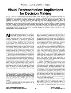
is still a challenging problem [18], many approaches have been proposed to solve it. A classical approach is to use a central catadioptric omnidirectional camera [24] and warp the image plane onto a unit sphere using the Geyer and Barreto’s model given in [14], [5]. Multiple cameras systems such as [25] permit construction of high resolution spherical views and rely on image stitching algorithms [28] but they assume the translation between each camera’s center of projection to be negligible with respect to the observed scene. Commercial off-the-shelf systems ensuring such a constraint, like LadyBug camera, can also be found. As we aim to focus on the loop closure issue, we do not detail the construction of the spherical views here. Using spherical views (Figure 1) provides several

Figure 1. Exemple of spherical view with SIFT interest points.

advantages to tackle the loop closure problem. Due to its shape -round, smooth and regular- the sphere is well adapted to register the scene structure. In term of image processing, visual features can be tracked a longer time before leaving the field of view. Besides the good properties provided by its shape, spherical view usually leads to a well-conditioned localization problem thanks to the observation of features homogeneously distributed around the viewpoint (Figure 2). They usually allow to define a one-toone mapping between a place and its corresponding observation, property of importance for topological localization. Finally, as the spherical views are invariant under the rotations around the center of projection, they are good candidates to support structure descriptors based on distribution of features over the sphere.

2.1. Spherical representation Using full 360◦ images like spherical views as an egocentered representation of the world has already proved its power and utility in user friendly applications such as Google Street View [31], and more recently [16]. Although building a spherical view with a unique center of projection

2.2. Structure enhancement - distribution registration In order to relate the sphere structure and the environment in a statistical way, we propose a novel representation based on the neighborhood notion directly defined on the

(a) Well conditioned sphere

(b) Ill conditioned sphere

Figure 2. Two top views of sphere used for topological localization. (a) Usual case with features all around the current position leading to a good localization. (b) Rare cases of ill-conditioned situations can occur if the features are located at the front and rear of the robot, for example, in a poorly textured corridor.

sphere. This representation preserves some suitable properties like the spherical view invariance to the rotations and guarantees a good robustness to occlusions due to, for instance, dynamic objects in the scene. We consider a set of local features (SIFT points in this paper) extracted on the sphere and, besides the feature based descriptor associated to the detector, we attach to each feature a novel descriptor based on a local histogram that characterizes the features distribution over the sphere. To compute this histogram, the sphere is divided into concentric rings centered on the current feature. Each bin corresponds to a sphere ring in which we register the number of features detected inside the ring. As we don’t take into account the feature descriptors, the histogram only represents feature density. There are as many distribution histograms as features detected in the topological place. Figure 3 shows a sphere discretization example. The sphere quantization level is an important parameter as it should be related to the feature density. Too large bins will loose some information about the features distribution: distribution will be too smoothed to be discriminant; whereas too small bins will be too much discriminative and won’t allow correct distribution comparisons due to quantization noise effect. The bins size is determined by a solid angle located at the sphere center. In our experiments, we found out that an angle of about 8◦ (24 bins) leads to the best results. Further investigation is presented in the results section. Our representation of the interest points therefore exploits two kinds of information, a locally defined visual information represented by the SIFT descriptors and a globally defined statistical information represented by the feature distribution over the sphere.

Figure 3. Sphere discretization into rings centered on a feature. The feature orientation is represented by the red segment from the sphere center to the feature location onto the sphere surface.

2.3. Codebook and inverted index file Visual vocabularies and inverted index files are chosen for representing the data. The codebook dynamically stores the visual words extracted from the images; using the SIFT detector. The inverted index stores for each visual word the places where it has been seen. Each place information for each word is enhanced with the feature density information. The codebook data structure must be flexible to easily store new words incrementally. Linear codebooks could be sufficient for small environment mapping but rapidly become intractable as the number of words increases. Our approach deals with large environments and thus implies codebooks with a huge amount of words (about 300 000 in our case) learned inline. To be efficient, the algorithm must use data structures with quick nearest neighbor search systems. Our codebook data structure is a standard unbalanced kd-tree that satisfies efficiency requirements and incremental storing needs. As we use an incremental data structure, visual words must be compared in order to determine if they are new words or if they are already stored in the codebook. Two words are compared using the euclidean distance. If the distance is small (under 0.22 in our experiments) the words are equal.

3. Loop closure detection 3.1. Bayesian filtering The bayesian loop closure detection algorithm presented in [2] constitute our algorithm basis. It could be summarized by the following formula: p(St |zt ) = η p(zt |St ) p(St |zt−1 ) | {z } | {z } | {z } term1

term2

term3

(1)

where St is the random variable representing the loop closure hypotheses at time t and zt is the set of all the visual words encountered until time t. Without describing the whole algorithm, term1 is the full posterior and will finally determine if a loop closure has occurred. term3 is computed as follows: t−p

p(St |zt−1 ) =

∑

p(St |St−1 = j)p(St−1 = j|zt−1 )

(2)

j=−1

where p(St |St−1 = j) is a time evolution model which gives the transition probability from one state at time t − 1 to every possible state at time t (more details can be found in [2]). p(St−1 = j|zt−1 ) is the loop closure probability at time t − 1 computed one step before. term2 is the likelihood function L(St |zt ) and corresponds to the similiraty evaluation between different places. The similarity evaluation relies on a scoring system in which the current place is compared with all already visited places using the visual words. The more the visual words are common between two images, the higher the score is. In order to compute those scores, [2] uses the classical t f id f scoring system presented in [27]. For each visual word w in current image and each image i containing w, the t f id f score is computed as follows: t f id f =

N nwi log( ) ni nw |{z} | {z } tf

(3)

id f

The term nwi is the number of visual words w in image i, ni is the number of visual words in image i. N is the number of places already visited and nw is the number of places where the word w appears in. Once the scores are computed, they are normalized and thresholded to create the likelihood function. As will be presented in the next section, we propose to modify this scoring system to take into account all the information extracted from the spherical representation, i.e. local and global information. Note that in [2], many false loop closures detected by the algorithm are filtered using epipolar constraints. The method presented here is purely qualitative and does not use epipolar geometry nor any kind of filter, but focuses on the reduction of false alarm rate prior to these verification.

3.2. Likelihood computation In our approach, local features, i.e. SIFT, are enhanced by the surrounding distribution of features over the sphere. Consequently, similar SIFT descriptors in a given image will be distinct due to their surrounding. The t f term denoting the frequency of a same feature used in the original approach will therefore become obsolete as it would have led to a t f term constantly equal to 1/ni . Therefore, we create a new scoring system called ts id f . The id f term is kept because, even if the distribution of

words around two corresponding visual words are identical, less seen words over images are more discriminative than the frequently seen ones. The ts term is a similarity measure between the feature density descriptors of two matching visual words. It denotes the importance relatively to structure consistency between places, i.e. the importance of having the same feature distribution around the compared features. tswi represents the structure consistency and is computed using the Tanimoto coefficient [30]. This coefficient computes the similarity between two distributions. tswi =

< histwc .histwi > khistwc k2 + khistwi k2 − < histwc .histwi >

(4)

< A.B > denotes the inner product of vectors A and B. histwc is the distribution histogram for word w in the current place and histwi is the distribution histogram of the same word in place i. The likelihood is computed as follows: visual words extracted from the current image are compared with the ones stored in the codebook. If a word already exists, places where it has been seen are retrieved from the inverted index file. For each of those places, the ts id f score is computed using the distribution histogram associated to the visual word - place pair. Once all the scores are computed, they are normalized and thresholded. The new scoring computation for a word w in current place and a place i containing w is therefore: ts id fwi = tswi log(

N ) nw

(5)

The total score computation for each place i is: ts id fi =

w

w

w∈i

w∈i

N

∑ ts id fwi = ∑ tswi log( nw )

(6)

3.3. Integral on full posterior Classical approaches use a threshold on the full posterior probability density function to determine if a loop closure occurs. This threshold can be considered as a confidence factor. Nevertheless, loop closing places are similar to nearby places. This results in a flattened gaussian like probability function around the index of the matching place with no loop closure detection (maximum of the curve under the threshold). Withal, it seems obvious that the flattened curve denotes a loop closure where the value is the higher. To overcome this issue, flattened curves are detected and replaced with strong peaks representing the local integral values. Then, the threshold is applied to these locally integrated curves. This solution improves the system reliability by decreasing the number of undetected loop closures. The curve detection is performed by applying a threshold slightly greater than 0- to determine the beginning and the ending of the curves.

Figure 5. Examples of localizations given by the algorithm. The left column contains current places and the right column contains the matching places. First five rows are correct topological localizations whereas the last row presents a false alarm example.

4. Experimental results Our approad has been tested on a 1.5 kms dataset acquired at INRIA Sophia Antipolis Research Center. The dataset is composed of about 1500 images of buildings and vegetation. The images are acquired by our multi perspective camera system shown in the figure 4 and precomputed to construct the spherical representation (the perspective images are projected onto a sphere located at the intersection point of the six camera optical axes). The acquisition system is made up of six perspective wide angle cameras on a ring. The images present some reprojection errors

implying some visual inconsistencies (bad stitching at the images intersections) due to the system configuration that has no unique optical center. Our experiments will focus on the loop closure detection algorithm robustness in the topological localization and mapping context. Loop closure query tests We first present some loop closure detection tests to illustrate the properties of our approach. Figure 5 shows some results for similarity queries from the current image. Correct loop closure detections in opposite directions are presented in the first three rows.

0.9 Spherical View, 24 bins Perspective Camera No epipolar constraint

0.8 0.7

True Positive Rate

0.6 0.5 0.4 0.3 0.2 0.1 0

Figure 4. Multi-camera system mounted on a electrical vehicle CyCab.

First row demonstrates the loop closure detection capability for good localization in environments with strong similarity like a parking. The second one shows localization in an environment with buildings like urban environments. The third one highlights the loop closing ability in environments with a lot of vegetation. Fourth row is an instance of time varying environment with dynamic objects (here a car). The fifth row is a case of loop closure detection with perpendicular point of views. This example is of particular interest as it highlights the algorithm performance for loop closure detection independently of the vehicle orientation. The last row is a place where the algorithm erroneously found a matching place. The presented instances are a small part of the dataset but are very representative of the loop closure detection algorithm. It is able to manage a large variety of environments even difficult ones such as vegetation or strong similarity. Most of the time the algorithm gives the good answer but it sometimes fails for the places where vegetation constitute an important part of the environment. This is partly due to the fact that lots of visual words are detected in the vegetation. Such visual words are not very informative and can roughly be considered as noise relatively to other visual words located on buildings, cars or roads. In Figure 6, our method is compared to the method presented in [2] where a standard perspective camera is used. One of the front camera mounted on our robot is used as a perspective camera and generates perspective images for the INRIA dataset. The presented algorithm obviously outperforms the one using only one perspective camera thanks to its ability to detect loop closures under varying point of view. On the curve representing the method with a standard perspective camera, the false positive rate should not be taken into account as epipolar constraints verification is not performed contrarily to the original algorithm. Epipolar constraints verification

0

0.1

0.2

0.3 0.4 0.5 False Positive Rate

0.6

0.7

0.8

Figure 6. Comparison between spherical view and standard perspective camera

allows a strong reduction of the false positive rate. The important observation is that the algorithm is unable to have a correct true positive rate. Methods using perspective cameras are unable to deal with such datasets as they are only able to detect loop closures under same point of view conditions, which are cases in the presented dataset. Interest of feature density histograms Without the exploitation of the feature density information, the algorithm naturally tends to find lots of loop closing places. Most of correct matches are detected but many incorrect matches are also detected (see the SIFT Only curve in Figure 7). Our solution involves the feature distribution over space to enhance the places distinctiveness. The ROC curve (24 bins for optimized results) in Figure7 points out the algorithm ability to detect true loop closures while not detecting too much false loop closures. The wrong matches are a problem as they destroy the topological map consistency; this issue can be overcome using stronger validating systemss such as Epipolar constraints. This constraint is often stated as necessary to reduce the rate of false loop closures. We did not add this constraint as it goes against our aim of studying an algorithm without any metric computation. The results are shown in the video1 . Study of the sphere discretization The number of rings dividing the sphere, i.e. the discretization parameter, impacts the algorithm ability to detect loop closures. Figure 7 points out the effects of this parameter. The TPR (true positive rate) falls as the number of bins increases (small rings). The distribution is over sampled and sensitive to the discretization noise. The comparison between distributions is not possible anymore. It explains the poor performance of the algorithm in this case and the low TPR observed. 1 https://www-sop.inria.fr/arobas/videos/loopclosure/

1 0.9

True Positive Rate

0.8

0.7 0.6

0.5 0.4

SIFT Only (No density descriptor) 10 bins 24 bins 40 bins

0.3 0.2

0

0.05

0.1

0.15 0.2 0.25 False Positive Rate

0.3

0.35

0.4

Figure 7. Sphere discretization impact on the robustness

When the number of bins decreases (large rings), the TPR increases at the cost of an increase of the FPR (false positive rate). The distribution is under sampled and consequently not enough disciminative. This results in a better TPR but also in an important increase of the FPR. We can observe the best compromise between TPR and FPR around a discretization of 24 bins. Algorithm performance Our algorithm runs online at the frequency of 1 Hz. The program is implemented in C++ and executed on two Intel Xeon E5540 with 16GB of RAM. The implementation does not actually take advantage of the multiprocessor system and runs on only one core. The average computation time for one image is 413 ms and the maximum required time observed is 656 ms. Figure 8. Drift correction using loop closures

Drift reduction Figure 8 shows the loop closure detection benefits in metrical trajectories estimation. Top image is the estimated trajectory followed by our electrical vehicle in the campus. The estimation is based on visual odometry only without loop closure detection [21]. The start point and the end point should be at the same place (ground truth). Middle image is the corrected trajectory using loop closures provided by the presented algorithm. Drift correction is performed using TORO [13], it optimizes the graph of poses with the loop closure constraints. The start point and the end point are corresponding. Bottom image details loop closures detected from perpendicular points of view.

5. Conclusion and future work Our method aims at dealing with large scale environenments in the context of apperance only based topological SLAM. Our main contributions are the spherical view exploitation to represent the environment structure and the design of a view point independent loop closure detection

algorithm. Moreover, the algorithm runs in real time with no a priori information (the codebook is built inline) and does not compute any metric information. We demonstrate the approach efficiency on large and complex environment made up of buildings and vegetation. The method still shows some drawbacks but presents some interesting results concerning the performance obtained for a qualitative system in a large scale environment. Further investigation will be led on the sphere exploitation in order to increase the algorithm robustness and reach a null false positive rate if possible. As the feature density descriptor robustness relies on the local descriptor robustness, tests will be performed using other local detectors. We will also try to use the feature density descriptor in a filtering phase. In the current model, it enhances the information provided by the local descriptors in order to have a more relevant similarity measure. The other way is to use the classical t f id f scoring system with a weak decision threshold for loop closure detection. This

would reduce the false negative rate. The feature density descriptor could then be used to filter the false positive loop closures instead of the epipolar constraint verification.

[15] T. Tuytelaars H. Bay and L. Van Gool. Surf: Speeded up robust features. In Computer Vision ECCV 2006, Lecture Notes in Computer Science, chapter 32, pages 404–417. 2006. 2

References

[16] R. Szeliski J. Kopf, B. Chen and M. Cohen. Street slide: Browsing street level imagery. ACM Transactions on Graphics (Proceedings of SIGGRAPH 2010), 29(4):to appear, 2010. 2

[1] J.-A. Meyer A. Angeli, S. Doncieux and D. Filliat. Incremental vision-based topological slam. In Intelligent Robots and Systems, 2008. IROS 2008. IEEE/RSJ International Conference on, pages 1031–1036, Sept. 2008. 2 [2] J.-A. Meyer A. Angeli, S. Doncieux and D. Filliat. Real-time visual loop-closure detection. In ICRA, pages 1842–1847. IEEE, 2008. 1, 3, 4, 6 [3] R. Anati A. Kumar, J.-P. Tardif and K. Daniilidis. Experiments on visual loop closing using vocabulary trees. In Computer Vision and Pattern Recognition Workshops, 2008. CVPRW ’08. IEEE Computer Society Conference on, pages 1 –8, 2008. 1, 2

[17] J. D. Chen P. Mihelich M. Calonder V. Lepetit P. Fua K. Konolige, J. Bowman. View-based maps. In Proceedings of Robotics: Science and Systems, Seattle, USA, June 2009. 1, 2 [18] G. Krishnan and S. K. Nayar. Towards A True Spherical Camera. In SPIE Human Vision and Electronic Imaging, Jan 2009. 2 [19] D. Lowe. Distinctive image features from scale-invariant keypoints. International Journal of Computer Vision, 60(2):91, November 2004. 2

[4] A. Angeli, D. Filliat, S. Doncieux, and J.-A. Meyer. A fast and incremental method for loop-closure detection using bags of visual words. IEEE Transactions On Robotics, Special Issue on Visual SLAM, 2008. 2

[20] J. J. Leonard M. Bosse, P. M. Newman and S. Teller. SLAM in Large-scale Cyclic Environments using the Atlas Framework. The International Journal of Robotics Research, 23(12):1113–1139, December 2004. 1

[5] J.P. Barreto. General central projection systems, modeling, calibration and visual servoing. PhD thesis, University of Coimbra, Dept. of Electrical and Computer Engineering, 2003. 2

[21] A.I. Comport M. Meilland and P. Rives. Dense visual mapping of large scale environments for real-time localisation. In Submitted to IEEE Conference on Intelligent Robots and Systems, IROS’11, San Fransisco, USA, September 2011. 7

[6] M. J. Cummins and P. M. Newman. Fab-map: Probabilistic localization and mapping in the space of appearance. I. J. Robotic Res., 27(6):647–665, 2008. 1, 2

[22] A. C. Murillo and J. Kosecka. Experiments in place recognition using gist panoramas. In Computer Vision Workshops (ICCV Workshops), 2009 IEEE 12th International Conference on, 27 2009. 1

[7] O. Naroditsky D. Nist´er and J. R. Bergen. Visual odometry. In CVPR (1), pages 652–659, 2004. 1 [8] A. J. Davison. Real-time simultaneous localisation and mapping with a single camera. In ICCV, pages 1403–1410. IEEE Computer Society, 2003. 1 [9] T. Maeda E. Menegatti and H. Ishiguro. Image-based memory for robot navigation using properties of omnidirectional images. Robotics and Autonomous Systems, 47(4):251–267, 2004. 1, 2 [10] V. Lepetit E. Tola and P. Fua. Daisy: An efficient dense descriptor applied to wide baseline stereo. IEEE Transactions on Pattern Analysis and Machine Intelligence, 99(1), 2009. 2 [11] T. Duckett F. Dayoub and G. Cielniak. An adaptive spherical view representation for navigation in changing environments. European Conference on Mobile Robots, 2009. 1 [12] C. Engels F. Fraundorfer and D. Nist´er. Topological mapping, localization and navigation using image collections. In IROS, pages 3872–3877. IEEE, 2007. 1 [13] C. Stachniss P. Pfaff G. Grisetti, S. Grzonka and W. Burgard. Efficient estimation of accurate maximum likelihood maps in 3d. In IROS, pages 3472–3478. IEEE, 2007. 7 [14] C. Geyer and K. Daniilidis. Catadioptric projective geometry. International Journal of Computer Vision, 45:223–243, 2002. 2

[23] J. Ostrowski L. Goncalves P. Pirjanian N. Karlsson, E. Di Bernardo and M. E. Munich. The vSLAM algorithm for robust localization and mapping. In 2005 IEEE International Conf. on Robotics and Automation, ICRA 2005, 2005. 1 [24] S. K. Nayar. Catadioptric omnidirectional camera. pages 482 –488, jun. 1997. 2 [25] Y. Aloimonos P. Baker, C. Fermuller and R. Pless. A spherical eye from multiple cameras. In IEEE Conference on Computer Vision and Pattern Recognition, 1:576, December 2001. 2 [26] E. Rosten and T. Drummond. Machine learning for highspeed corner detection. In European Conference on Computer Vision, volume 1, pages 430–443, May 2006. 2 [27] J. Sivic and A. Zisserman. Video google: A text retrieval approach to object matching in videos. In ICCV, pages 1470– 1477. IEEE Computer Society, 2003. 4 [28] R. Szeliski. Image alignment and stitching: a tutorial. Found. Trends. Comput. Graph. Vis., 2(1):1–104, 2006. 2 [29] T. Tuytelaars T. Goedem´e, M. Nuttin and L. Van Gool. Omnidirectional vision based topological navigation. International Journal of Computer Vision, 74(3):219–236, 2007. 1 [30] T. T. Tanimoto. IBM Internal Report, 1957. 4 [31] L. Vincent. Taking online maps down to street level. Computer, 40:118–120, 2007. 2