A splitting method for separate convex ... - Optimization Online

A splitting method for separate convex programming with linking linear constraints Bingsheng He1

Min Tao2

and

Xiaoming Yuan3

June 25, 2010 Abstract. We consider the separate convex programming problem with linking linear constraints, where the objective function is in the form of the sum of m individual functions without crossed variables. The special case with m = 2 has been well studied in the literature and some algorithms are very influential, e.g. the alternating direction method. The research for the case with general m, however, is in completely infancy, and only a few methods are available in the literature. To generate a new iterate, almost all existing methods produce temporary iterates via solving m subproblems generated by splitting the corresponding augmented Lagrangian function in either parallel or alternating way, and then apply some correction steps to correct the temporary iterates. These correction steps, however, may result in critical difficulties for some applications of the model under consideration. In this paper, we develop the first method requiring no correction steps at all to generate new iterates for the model with general m. We also apply the new method to solve some concrete applications arising in image processing and Statistics, and report the promising numerical performance. Keywords: Convex programming, separate structure, linking constraint, augmented Lagrangian method, total variation, image restoration

1

Introduction

We consider the separate convex programming problem with linking linear constraints, where the objective function is in the form of the sum of m individual functions without crossed variables: (m ) m X X min (1.1) θi (xi ) | Ai xi = b; xi ∈ Xi , i = 1, 2, . . . , m , i=1

i=1

where θi : 0 is the Gaussian noise level and k · kF is the standard Frobenius norm. As in [48], we let C = A∗ + E ∗ be the data matrix, where A∗ and E ∗ are the low-rank and sparse components to be recovered, respectively. We generate A∗ by A = LRT , where L and R are independent m × r matrices whose elements are i.i.d. Gaussian random variables with zero means and unit variance. Hence, the rank of A∗ is r. The index of observed entries, i.e. Ω, is determined at random. The support Γ ⊂ Ω of the impulsive noise E ∗ (sparse but large) are chosen uniformly at random, and the non-zero entries of E ∗ are i.i.d. uniformly in the interval [−500, 500]. Let sr, 15

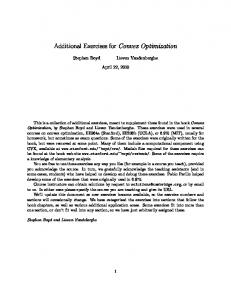
spr and rr represent the ratios of sample (observed) entries (i.e., |Ω|/mn), the number of non-zero entries of E (i.e., kEk0 /mn) and the rank of A∗ (i.e., r/m), respectively. To witness the fact that correction steps are likely to destroy the low-rank characteristic of the recovered low-rank component, we focus on the special case of (5.2) with √ δ = 0, τ = 1/ n, m = n = 500, rr = spr = 0.05 and sr = 0.6. We executed the singular value decomposition (SVD) fully to compute the exact ranks of the recovered low-rank components Ak , and recorded the variation of the ranks for Algorithm 1 and the ADBC method in the following figure (left). Evolution of rank(Ak) for Algo. 1 and ADBC

Errors of Algorithm 1 and ADBC 1

Algo. 1 ADBC

70

Algo. 1: errsSP Algo. 1: errsLR ADBC: errsSP ADBC: errsLR

0.9

65 0.8

60 0.7

55 rank

0.6

50

0.5

45

0.4

40

0.3

35

0.2

30

0.1

25 0

20

40

60 80 Iteration number

100

120

0 0

140

20

40

60 80 Iteration number

100

120

140

Figure 1: Evolution of rank (left) and errors of recovered components (right) for Algorithm 1 and ADBC As shown in Figure 1, the rank of iterates generated by ADBC changes radically according to iterations at the first stage; while the rank of iterates generated by Algorithm 1 is much more stable— not sensitive to the iterations. We believe that the reason behind this difference is that the correction step of ADBC destroys the underlying low-rank feature. On the opposite, the low-rank feature is well preserved by Algorithm 1; and this merit is very suitable for the application of some popular packages for partial SVD such as PROPACK. For exposing the difference resulted by correction steps, we also compare their respective variations of the recovered low-rank component’s error and sparse component’s error denoted by errsLR :=

kAk − A∗ kF kA∗ kF

and errsSP :=

kE k − E ∗ kF kE ∗ kF

in the right of Figure 1. As shown clearly, compared to Algorithm 1, the errors generated by ADBC’s iterations, especially the recovered low-rank component’s error, change more radically. Therefore, Figure 1 illustrates well our motivation of presenting such an splitting algorithm without any correction steps for solving (1.1).

5.2

The efficiency of Algorithm 1

In this subsection, we mainly show the efficiency of the proposed Algorithm 1 to solve some applications of (1.1) arising in the area of image processing. We also implement the proposed Algorithm 2 in this subsection. With the comparison of Algorithms 1 and 2, the reason of avoiding correction steps is further justified. 16

As delineated in [26], the model (1.1) captures many important applications of digital image restoration and reconstruction problems arising in image processing. Digital image restoration and reconstruction problems play an important role in various areas of applied sciences such as medical and astronomical imaging, film restoration and image and video coding and many others. Let 2 2 2 2 2 x ¯ ∈ Rn be the original image, K ∈ Rn ×n be a blurring (or convolution) operator, S ∈ Rn ×n be a diagonal matrix, which diagonal entry is 0 (i.e. missing the corresponding information) or 1 (i.e. 2 2 keeping the corresponding information), ω ∈ Rn be an additive noise, and f ∈ Rn which satisfies the relationship f = SK x ¯ + ω. (5.3) Given S, K, our objective is to recover x ¯ from f , which is known as the problem of image inpainting. When S is the identity operator, recovering x ¯ from f is referred to as deconvolution. It is well known that (5.3) is an ill-conditioned problem. To stabilize the recovery, one must utilize some prior information such as adding a regularizer to certain data fidelity. The total variation (TV) regularization introduced in [43] for image construction has been shown both experimentally and theoretically to be suitable for preserving sharp edges. More specifically, denote the discrete gradient 2 2 2 2 operators as ∂1 : Rn → Rn and ∂2 : Rn → Rn , which represent the discretized derivatives in the horizontal and vertical directions, respectively. The gradient operator is then defined as ∇ := (∂1 , ∂2 ). Then the TV inpainting model can be formulated as the following reconstruction model µ (5.4) min k|∇x|k + kSKx − f kN , x 2 or the equivalent constrained form: min k|∇x|k 2 s.t. x ∈ Rn , kSKx − f kN ≤ α.

(5.5)

Ã

! p y1 2 2 2 Here, let y = ∈ Rn × Rn , we define |y| = y12 + y22 ∈ Rn , and k · kN refers a norm, in y2 particular k · k2 = k · k. The parameter α is positive real numbers, which measures the trade-off between the fit to f and the amount of regularization. In this following, we apply both the proposed methods to solve the constrained TV-l2 model, i.e., let N = 2 in (5.5), which is to restore a blurred image with additive Gaussian noise. To ensure the nonempty of the solution set, we assume that the constraint set 2

Ω := {x ∈ Rn , kSKx − f k ≤ α}

(5.6)

is nonempty. First, we rewrite the problem (5.5) into: min k|y|k s.t. y = ∇x, Kx = z, z ∈ Z,

(5.7)

where 2

Z := {z ∈ Rn , kSz − f k ≤ α} is a ball. Then, (5.7) is a special case of (1.1) where 2

2

x = (x1 , x2 , x3 ) = (y, x, z) ∈ R2n × Rn × Z 17

f1 (y) = k|y|k, f2 (x) = 0, f3 (z) = 0 and

à A = (A1 , A2 , A3 ) =

! I −∇ 0 0 −K I

Ã

! 0 0

and b =

.

The augmented Lagrangian functional associated to this problem is defined by 1 1 L(x, y, z, λ1 , λ2 ) = k|y|k1 − λT1 (y − ∇x) − λT2 (z − Kx) + ky − ∇xk2H + kz − Kxk2H . 2 2 To expose the main idea clear, throughout we set H ≡ βI and we restrict out discussion into the case where β > 0 is fixed. Now, we elaborate on the strategy of solving the resulted subproblems when the proposed Algo˜k , x rithm 1 is applied to solve (5.7). Recall that we denote by (˜ yk , λ ˜k ), z˜k the iterate generated by Algorithm 1 for solving (5.7). • The first subproblem (3.1) amounts to solving y˜k ∈ argmin y k|y|k1 +

β 1 ky − ∇xk − λk1 k2 . 2 β

Obviously, the closed-form solution of the above minimization problem is given by µ ¶ λk y˜k = shrink 1 ∇xk + 1 , β β Ã ! y1 2 2 ∈ Rn × Rn and a scalar β > 0, the operator shrinkβ (y) is where for a vector y = y2 defined as y shrinkβ (y) = y − min(β, |y|) · , (5.8) |y| p 2 where |y| ∈ Rn be defined by |y| = y12 + y22 and 0 · (0/0) = 0 is assumed. • The second subproblem (3.2) is trivial whenever y˜k is computed. • The third subproblem (3.3) amounts to solving x ˜k ∈

k+ 1 argmin x (λ1 2 )T ∇x

+

k+ 1 (λ2 2 )T (Kx)

β + µk 2

Ã

! −∇ −K

(x − xk )k2 ,

whose solution can be obtained via solving the following system of linear equations: k+ 12

βµ(∇T ∇ + K T K)(˜ xk − xk ) = −∇T λ1

k+ 12

− K T λ2

.

(5.9)

Assuming that the blur K is spatially invariant and periodic boundary conditions are used for the discrete differential operator, we see that the matrices K and ∇T ∇ can be diagonalized by the Fast Fourier transform (FFT).

18

• The fourth subproblem (3.4) amounts to solving k+ 12 T

z˜k ∈ argmin z (−λ2

) z+

β µkz − z k k2 , 2

whose closed-form solution is given by: z˜k = PB [z k +

1 k+ 1 λ 2 ]. βµ

Here the projection operator PB (·) is defined as PB (t) =

t−f . ∗ min(kt − f k, α) + f, kt − f k

2

where t ∈ Rn . In the following, we implement both Algorithms 1 and 2 to the Lena image (256×256). The iteration will be terminated whenever kxk+1 − xk k < ², max{kxk k, 1}

(5.10)

where ² > 0 is a given tolerance. As usually used, we measure the quality of restoration by the signal-to-noise ratio (SNR), which is measured in decibel (dB) and defined by SNR(x) , 10 ∗ log10

k¯ x−x ˜k2 , k¯ x − xk2

(5.11)

where x ¯ is the original image and x ˜ is the mean intensity value of x ¯. In the following experiments, Guassian kernel was applied with blurring size hsize = 5, standard deviation σ = 14 under two cases: one is noise level std = 10−3 with 40% information, the other is noise level std = 10−2 with 30% information. We set the missing pixels as 0. We set ² = 5 × 10−3 , α = kKx − f k, and µ = 1.8, γ = 1.3, β = 18. In Figure 2, we present the destroyed image and recover results from two methods in terms of relative error, SNR, consuming time (CPU) and iteration numbers (It.).

6

Conclusions

For solving the separate convex programming problem with linking linear constraints whose objective function is in the form of the sum of m individual functions without crossed variables, we present the first splitting algorithm where m smaller and easier subproblems are solved separately at each iteration and no any correction steps are required. The superiority and efficiency of the new method is illustrated by some numerical examples. At each iteration of the new method, however, the resulted m subproblems are not suitable for completely simultaneous computation as the latter m − 1 subproblems require the solution of the first subproblem. With the consideration of using advanced computing infrastructure such as parallel facilities, it is of interest to develop such a splitting algorithm whose resulted subproblems at each iteration are completely tailored for simultaneous computation. This is one of our research topics in the future.

19

B. & N., RE: 77.56%

RE: 6.88%, SNR: 15.07dB, CPU= 2.7s, It.: 42

RE: 6.47%, SNR: 15.60dB, CPU= 4.3s, It.: 47

B. & N., RE: 83.83%

RE: 7.49%, SNR: 14.33dB, CPU= 3.2s, It.: 51

RE: 7.27%, SNR: 14.59dB, CPU= 5.0s, It.: 59

Figure 2: Recovered results from Algo. 1 and 2 on TV-l2 . In both rows from left to right: blurry and noisy image missing partial information (B. & N.) and recovered results from Algorithm 1. and 2., respectively. RE, CPU and It. represent relative error, running time and iteration numbers, respectively. Top row: std = 10−3 and lost 60% information; Bottom row: std = 10−2 and missing 70% information.

20

References [1] M. V. Afonso, J. M. Bioucas-Dias and M. A. T. Figueiredo, Fast image recovery using variable splitting and constrained optimization, manuscript, 2009. [2] A. Auslender and M. Teboulle, Entropic proximal decomposition methods for convex programs and variational inequalities, Math. Program., 91, 33-47, 2001. [3] D. P. Bertsekas, Constrained Optimization and Lagrange Multiplier methods, Academic Press, 1982. [4] E. Blum and W. Oettli. Mathematische Optimierung. Springer-Verlag, Berlin, 1975. Grundlagen und Verfahren, Mit einem Anhang “Bibliographie zur Nichtlinearer Programmierung”, ¨ Okonometrie und Unternehmensforschung, No. XX. [5] N. Bose and K. Boo, High-resolution image reconstruction with multisensors, International Journal of Imaging Systems and Technology, 9, 294-304, 1998. [6] E. J. Cand` es, X. Li, Y. Ma and J. Wright, Robust Principal Component Analysis, manuscript, 2009. [7] Y. Censor, T. Elfving, N., Kopf and T. Bortfeld, The multiple-sets split feasibility problem and its applications for inverse problems, Inverse Problems, 21, 2071-2084, 2005. [8] V. Chandrasekaran, S. Sanghavi, P. A. Parrilo and A. S. Willskyc, Rank-sparsity incoherence for matrix decomposition, manuscript, http://arxiv.org/abs/0906.2220. [9] G. Chen and M. Teboulle, A proximal-based decomposition method for convex minimization problems, Mathematical Programming, 64, 81-101, 1994. [10] P. L. Combettes and J.-C. Pesquet, Proximal splitting methods in signal processing, in: FixedPoint Algorithms for Inverse Problems in Science and Engineering, (H. H. Bauschke, R. Burachik, P. L. Combettes, V. Elser, D. R. Luke, H. Wolkowicz, Editors), New York: SpringerVerlag, 2010. [11] J. Douglas and H. H. Rachford, On the numerical solution of the heat conduction problem in 2 and 3 space variables, Transactions of the American Mathematical Society, 82, 421-439, 1956. [12] J. Eckstein, Some saddle-function splitting methods for convex programming, Optimization Methods and Software, 4, 75-83, 1994. [13] J. Eckstein and D. P. Bertsekas, On the Douglas-Rachford splitting method and the proximal points algorithm for maximal monotone operators, Math. Program., 55, 293-318., 1992. [14] J. Eckstein and B. F. Svaiter, General projective splitting methods for sums of maximal monotone operators, SIAM J. Control Optim., 48, 787-811, 2009. [15] E. Esser, Applications of Lagrangian-Based alternating direction methods and connections to split Bregman, UCLA CAM Report 09-31, 2009. [16] J. Eckstein and M. Fukushima, Some reformulation and applications of the alternating direction method of multipliers, Large Scale Optimization: State of the Art, W. W. Hager et al eds., Kluwer Academic Publishers, pp. 115-134, 1994. 21

[17] F. Facchinei and J.-S. Pang, Finite-Dimensional Variational Inequalities and Complementarity problems, Volume I, Springer Series in Operations Research, Springer-Verlag, 2003. [18] M. Fukushima, Application of the alternating direction method of multipliers to separable convex programming problems, Computational Optimization and Applications, 2, pp. 93-111, 1992. [19] D. Gabay and B. Mercier, A dual algorithm for the solution of nonlinear variational problems via finite-element approximations, Computer and Mathematics with Applications, 2, pp. 17-40, 1976. [20] D. Gabay, Applications of the method of multipliers to variational inequalities, Augmented Lagrange Methods: Applications to the Solution of Boundary-valued Problems, M. Fortin and R. Glowinski, eds., North Holland, Amsterdam, The Netherlands, pp. 299-331, 1983. [21] R. Glowinski, Numerical Methods for Nonlinear Variational Problems, Springer-Verlag, New York, Berlin, Heidelberg, Tokyo, 1984. [22] R. Glowinski and P. Le Tallec, Augmented Lagrangian and Operator-Splitting Methods in Nonlinear Mechanics, SIAM Studies in Applied Mathematics, Philadelphia, PA, 1989. [23] D. Goldfarb and S. Q. Ma, Fast alternating linearization methods for minimizing the sum of two convex functions, manuscript, 2009. [24] D. Goldfarb and S. Q. Ma, Fast multiple splitting algorithms for convex optimization, manuscript, 2009. [25] T. Goldstein and S. Osher, The split Bregman method for L1-regularized problems, SIAM J. Imaging Sciences, 2 (2), pp. 323-343, 2009. [26] D. R. Han, X. M. Yuan and W. X. Zhang, An augmented-Lagrangian-based parallel splitting method for linearly constrained separate convex programming with applications to image processing, submission, 2010. [27] B. S. He, Parallel splitting augmented Lagrangian methods for monotone structured variational inequalities, Computational Optimization and Applications, 42, 195-212, 2009. [28] B. S. He, L. Z. Liao, D. Han and H. Yang, A new inexact alternating directions method for monontone variational inequalities, Mathematical Programming, 92, 103-118, 2002. [29] B. S. He, M. Tao, M. H. Xu and X. M. Yuan, Alternating directions based contraction method for generally separable linearly constrained convex programming problems, Manuscript, 2009. [30] B. S. He, M. H. Xu and X. M. Yuan, Solving large-scale least squares covariance matrix problems by alternating direction methods, SIAM J. Matrix Analysis Appli., in revision. [31] M. Hestenes, Multiplier and gradient methods, J. Opti. Theory Appli., 4, 303-320, 1969. [32] K. C. Kiwiel, C. H. Rosa and A. Ruszczy´ nski, Proximal decomposition via alternating linearization, SIAM J. Opti., 9(3), 668-689, 1999. [33] S. Kontogiorgis and R. R. Meyer, A variable-penalty alternating directions method for convex optimization, Mathematical Programming, 83, 29-53, 1998. 22

[34] Z. K. Jiang and X. M. Yuan, A new parallel descent-like method for solving a class of variational inequalities, Journal of Optimization Theory and Applications, 145(2), 311-323, 2010. [35] Z.-C. Lin, M.-M. Chen, L.-Q. Wu, Y. Ma, The augmented Lagrange multiplier method for exact recovery of corrupted low-rank matrices, manuscript, 2009. [36] B. Martinet, Regularision d’in´equations variationnelles par approximations successive, Revue Francaise d’Automatique et Informatique Recherche Op´erationnelle, 126, 154-159, 1970. [37] M. Ng, F. Wang and X. M. Yuan, Fast minimization methods for solving constrained totalvariation superresolution image reconstruction, Multidimensional Systems and Signal Processing, to appear. [38] M. Ng, P. A. Weiss and X. M. Yuan, Solving constrained total-variation problems via alternating direction methods, SIAM J. Sci. Comput., to appear. [39] J. Nocedal and S. J. Wright, Numerical Optimization. Second Edition, Spriger Verlag, 2006. [40] M. Powell, A method for nonlinear constraints in minimization problems, in Optimization, R. Fletcher (Editor), pp. 283-298, Academic Press, New York, 1969. [41] R. T. Rockafellar, Monotone operators and the proximal point algorithm, SIAM J. Control Optim., 126, 877-898, 1976. [42] C. H. Rosa, Pathways of Economic Development in an Uncertain Environment: A Finite Scenario Approach to the U.S. Region under Carbon Emission Restrictions, WP-94-41, International Institute for Applied Systems Analysis, Laxenburg, Austria, 1994. [43] L. Rudin, S. Osher and E. Fatemi, Nonlinear total variation based noise removal algorithms, Physica D, 60, 259-268, 1992. [44] S. Setzer, Split Bregman algorithm, Douglas-Rachford splitting, and frame shrinkage, Lecture Notes in Computer Science, 5567, pp. 464-476, 2009. [45] S. Setzer, G. Steidl and T. Tebuber, Deblurring Poissonian images by split Bregman techniques, J. Visual Communication and Image Representation, 21, pp. 193-199, 2010. [46] J. E. Spingarn, Partial inverse of a monotone operator, Appl. Math. Optim., 10, 247-265, 1983. [47] J. Sun and S. Zhang, A modified alternating direction method for convex quadratically constrained quadratic semidefinite programs, manuscript, 2009. [48] M. Tao and X. M. Yuan, Recovering low-rank and sparse components of matrices from incomplete and noisy observations, SIAM J. Optim, in revision. [49] P. Tseng, Alternating projection-proximal methods for convex programming and variational inequalities, SIAM J. Optim., 7, 951-965, 1997. [50] Z. Wen, D. Goldfarb and W. Yin, Alternating direction augmented Lagrangian methods for semidefinite programming, manuscript, 2009. [51] Z. Wen, D. Goldfarb, A line search multigrid method for large-scale convex optimization, manuscript, 2007. 23

[52] J. Yang and Y. Zhang, Alternating direction algorithms for l1 -problems in compressive sensing, TR09-37, CAAM, Rice University. [53] C. H. Ye and X. M. Yuan, A descent method for structured monotone variational inequalities, Optim. Methods Softw., 22, 329-338, 2007. [54] X. M. Yuan, Alternating direction methods for sparse covariance selection, manuscript, 2009. [55] X. M. Yuan and J. Yang, Sparse and low rank sparse matrix decomposition via alternating directions method, manuscript, 2009.

24