A Stencil Compiler for Short-Vector SIMD Architectures Tom Henretty
Richard Veras
Franz Franchetti
The Ohio State University
Carnegie Mellon University
Carnegie Mellon University
[email protected]
[email protected]
[email protected]
Louis-Noël Pouchet
J. Ramanujam
P. Sadayappan
Univ. California, Los Angeles
Louisiana State University
The Ohio State University
[email protected]
[email protected]
[email protected]
ABSTRACT Stencil computations are an integral component of applications in a number of scientific computing domains. Short-vector SIMD instruction sets are ubiquitous on modern processors and can be used to significantly increase the performance of stencil computations. Traditional approaches to optimizing stencils on these platforms have focused on either short-vector SIMD or data locality optimizations. In this paper, we propose a domain-specific language and compiler for stencil computations that allows specification of stencils in a concise manner and automates both locality and short-vector SIMD optimizations, along with effective utilization of multi-core parallelism. Loop transformations to enhance data locality and enable load-balanced parallelism are combined with a data layout transformation to effectively increase the performance of stencil computations. Performance increases are demonstrated for a number of stencils on several modern SIMD architectures.
Categories and Subject Descriptors D.1.3 [Programming Techniques]: Concurrent Programming— Parallel Programming; D.3.4 [Programming Languages]: Processors—Code Generation, Compilers
Keywords DSL, Multicore, SIMD, Split Tiling, Stencils
1. INTRODUCTION There is increasing interest in developing domain-specific frameworks for high-performance scientific computing due to the diversity of current/emerging parallel architectures. In addition to the benefit of a DSL (Domain Specific Language) on user productivity, a significant advantage is that semantic properties derived from the high-level abstractions can be utilized to develop powerful specialized compiler transformations that can be tailored to the characteristics of different architectural platforms. Using the Stencil Domain Specific Language (SDSL) [11], this paper describes a set of compiler transformations that are needed to generate efficient code for
Permission to make digital or hard copies of all or part of this work for personal or classroom use is granted without fee provided that copies are not made or distributed for profit or commercial advantage and that copies bear this notice and the full citation on the first page. To copy otherwise, to republish, to post on servers or to redistribute to lists, requires prior specific permission and/or a fee. ICS’13, June 10–14, 2013, Eugene, Oregon, USA. Copyright 2013 ACM 978-1-4503-2130-3/13/06 ...$15.00.
multicore processors with short-vector SIMD ISAs such as SSE, AVX, VSX, LRBNi etc. Stencil computations involve arithmetic operations on physically contiguous data elements, e.g., c0*(A[i-1]+A[i]+A[i+1]). Since vector operations with ISAs like SSE require the loading of physically contiguous data elements from memory into vector registers and the execution of identical and independent operations on the components of vector registers, stencil computations pose challenges to efficient implementation on these architectures, requiring the use of redundant and unaligned loads of data elements from memory into different slots in different vector registers. We [12] had previously addressed this issue through a dimension-liftingtranspose (DLT) data layout transformation. However, only sequential execution was addressed. Further, the approach was only evaluated on data sets that fit in L1 cache. Tiling over spatial and the time dimensions is essential in conjunction with DLT for high performance on large data sets. However, as elaborated in detail in the next section, standard time-tiling of stencil codes via skewing introduces inter-tile dependences that are incompatible with the form of vector parallelism used by the DLT transformation. In this paper, we develop an integrated approach to perform tiling in conjunction with DLT transformation to generate efficient parallel code for stencil computations over large data sets on shared memory multiprocessors. We compare performance with code generated by the Pochoir stencil compiler [18] and Pluto [2, 4] for several benchmarks on multiple target multicore processors, demonstrating strong performance benefits for 1D and 2D stencils. The paper makes the following contributions: • It presents a stencil DSL compiler that integrates data layout transformation for short-vector SIMD ISAs with loadbalanced tiled parallel execution for multi-statement stencils. • It demonstrates significant performance improvement on several multi-core platforms for a number of benchmarks, over Intel’s ICC compiler and state-of-the-art research compilers like Pochoir and Pluto. The paper is organized as follows. In Sec. 2 we use an illustrative example to explain the main problem to be addressed in integrating DLT with tiling. Sec. 3.1 describes the stencil DSL and Sec. 3.4 provides a high-level overview of the compiler algorithms developed. Sections 4 and 5 provide details of the compiler algorithms. Experimental results are presented in Sec. 6 and related work is covered in Sec. 7.
2.
PROBLEM DESCRIPTION
In this section we first provide some background on the DLT data layout transformation of Henretty et al. [12] that was developed to overcome the fundamental data access inefficiency on current
short-vector SIMD architectures with stencil computations. We then describe why standard time-tiling is infeasible in conjunction with the DLT transformation and a different form of tiling – splittiling – can be used effectively in conjunction with DLT.
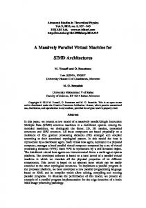
2.1 Overview of DLT Transformation Fig. 1 illustrates the DLT transformation for a one-dimensional vector of 24 elements for an ISA with a vector length of 4. Whereas B[0:3] form an aligned vector before transformation, after the DLT transformation, B[0], B[6], B[12], and B[18] form the first four elements Bdlt[0:3] in the transformed layout. The next four contiguous elements Bdlt[4:7] in the transformed layout correspond to B[1], B[7], B[13], and B[19], etc. Thus the sum of aligned vectors, Bdlt[0:3]+Bdlt[4:7]+Bdlt[8:11], computes < B[0] + B[1] + B[2], B[6] + B[7] + B[8], B[12] + B[13] + B[14], B[18] + B[19]+ B[20] >. Thus the fundamental problem with vectorized addition of contiguously located elements in memory is overcome in the transformed layout where operands that need to be combined are located in the same slot of different vectors rather than in different slots of the same vector. 0
1
2
3
0
1
2
3
0
1
2
3
0
1
2
3
0
1
2
3
0
1
2
3
A
B
C
D
E
F
G
H
I
J
K
L
M
N
O
P
Q
R
S
T
U
V
W
X
A
G
M
S
B
H
N
T
C
I
O
U
D
J
P
V
E
K
Q
W
F
L
R
X
(a) Original Layout
V N V
V
A
B
C
D
E
F
G
H
I
J
K
L
M
N
O
P
Q
R
S
T
U
V
W
X
N V
(b) Dimension Lifted
(c) Transposed
0
1
2
3
0
1
2
3
0
1
2
3
0
1
2
3
0
1
2
3
0
1
2
3
A
G
M
S
B
H
N
T
C
I
O
U
D
J
P
V
E
K
Q
W
F
L
R
X
(d) Transformed Layout
Stencil code: for (i = 1; i < 24; ++i) A[i] = B[i-1]+B[i]+B[i+1];
Figure 1: Data layout transformation for SIMD vector length of 4
2.2 Standard Tiling and DLT Transformation We next use a Jacobi 1D stencil example to explain the problem with the use of standard time-tiling in conjunction with DLT layout transformation. Although the input to our stencil compiler uses a special DSL language (described in Sec. 3.1), we use standard loop notation in C to motivate the problem since this lowerlevel view makes it easier to discuss issues pertaining to loop fusion and time-tiling when compiling general multi-statement stencils for high performance – something that to the best of our knowledge is not addressed by other stencil compilers such as PATUS [5] and Pochoir [18]. Fig. 2(a) shows code for a 1D Jacobi 3-point stencil with a sequence of two spatial loops within an outer time loop, where S1 performs the stencil computation over the spatial domain and S2 copies the output array into the input array for use in the next time step. In order to enhance data locality, time-tiling may be employed, but will first require some transformations in order to create atomic tiles that compute forward for several time steps over a subset of the spatial domain that is small enough to fit within cache. Fig. 2(b) shows a fused form that creates a unified 2D iteration
for (t=0; t δ = 1, δ =< 0 > T i T i Combining the dependence information from the DSG with the loop bounds of Fig. 12 gives us validity constraints on values the The spatial components of the distance vectors are then coaloop bounds may take, and results in the following system of inlesced into a tuple for each dependence such that the coalesced equalities for lower bounds: tuple C f s→ f t =< δL , δU > where δL is the maximum spatial distance and δU is the minimum spatial distance between two depenf2 ii + of1 L + α ∗ t ≤ ii + oL + α ∗ t − 1 dent statements f s and f t. For the Jacobi 1D example the tuples f2 ii + oL + α ∗ (t − 1) ≤ ii + of1 for each dependence are identical, Cf1→f2 = Cf2→f1 =< 1, −1 >. L +α∗t −1 These tuples are used to label edges in the DSG, along with a sepThe following system constrains the upper bounds: arate label for the time distance δT . Assembling the coalesced tuf1 f2 ples, time distances, dependences, and statements leads to the DSG ii + TU + oU + β ∗ t ≥ ii + TU + oU +β∗t +1 shown in Fig. 11 for the Jacobi 1D example. f2 f1 ii + TU + oU + β ∗ (t − 1) ≥ ii + TU + oU + β ∗ t + 1 Simplifying and rearranging these systems of inequalities yields the following system of difference constraints for lower bounds:
= !T = 0
Compute (f1)
Copy (f2)
f2 of1 L − oL
≤ −1
f1 of2 L − oL
≤ α − 1;
the corresponding constraints for upper bounds are shown below:
= !T = 1
f2 f1 oU − oU
≤
−1
f1 f2 oU − oU
≤
−β − 1.
These systems are used in Sec. 4.1.4 to compute valid offsets for all statements. Figure 11: Dependence Summary Graph (DSG) for Jacobi 1D
This DSG is subsequently used in Sec. 4.1.3 to build validity constraints for split-tiles and in Sec. 4.1.4 to compute slopes and statement offsets.
4.1.3
Building Validity Constraints
We seek to constrain the legal values of tile slope and statement offsets by assembling a system of linear inequalities based upon the DSG and the loop bounds of the split-tiled code we will generate. Pseudocode for the loop nests of Jacobi 1D upright tile is shown in Fig. 12. Informally, the validity constraints state that, for any pair of dependent statements, given a region over which the target
4.1.4
Computing Slopes and Offsets
To determine legal values for slopes α and β we compute, respectively, maximum and minimum cycle ratios [1, 7] on the DSG. A cycle ratio ρL (C) on the DSG is computed by finding a cycle C, summing δL values over the cycle, and dividing by the sum of δT values. A cycle ratio ρU (C) is calculated in a similar fashion with δU values. We set α = max(ρL (C)) and β = min(ρU (C)) for all cycles C in the DSG. We examine the only cycle in our example DSG, C0 , between f1 and f2. The DSG tells us that computing f1 on some interval [A, B] at time T allows us to compute f2 on the interval [A + f 1→ f 2 f 1→ f 2 f 1→ f 2 δL , B + δU ] at time T + δT without violating any dependences. Continuing along the cycle, computing f2 on the in-
f 1→ f 2
f 1→ f 2
f 1→ f 2
terval [A + δL , B + δU ] at time T + δT allows us to f 1→ f 2 f 2→ f 1 f 1→ f 2 + δL , B + δU + compute f1 on the interval [A + δL f 2→ f 1 f 1→ f 2 f 2→ f 1 δU ] at time T + δT + δT . Substituting in known values for the various δ variables shows us that computing f1 over the interval [A, B] at time T allows us to compute f1 over the interval [A + 2, B − 2] at time T + 1. Thus, we see a slope of 2 on the lower bound and a slope of -2 on the upper bound. Equivalently, summing δL values and dividing by the sum of δT values gives us ρL (C0 ) = 2; a similar calculation gives us ρU (C0 ) = −2. Since there is only one cycle in the DSG, these values are max(ρL (C)) and min(ρU (C)), and we set α = max(ρL (C)) = 2 and β = min(ρU (C)) = −2. These values for α and β are substituted into the systems of difference constraints, and a solution to each of these systems is obtained using the Bellman-Ford algorithm [1, 6]. For the Jacobi 1D f1 f2 f2 example we obtain of1 L = −1, oU = 1, and oL = oU = 0.
4.2 General Method Our general algorithm closely follows the principles we have explained for Jacobi 1D. Since stencils may be multidimensional slopes and offsets are separately computed for each dimension. Further, different stencil functions may apply to different subdomains, which may be disjoint, overlapping, or identical. Because of this we conservatively assume all stencil functions are executed at all points in the problem domain when calculating dependences. This is an over-approximation of data dependences and has no impact on the final correctness of the generated code. We present in Fig. 13 a general algorithm for computing slopes and offsets for a given input program. This algorithm produces lower/upper slope vectors with one slope per dimension, and lower/upper offset vectors with one offset per stencil statement. Input P: input SDSL program Output (~α, ~β, o~L , o~U ): Vectors of slopes alpha, beta. Vectors of lower and upper offsets in each spatial dimension for each stencil statement
D ← calculateDependences(P) s ← calculateDependenceDistances(D ) DSG ← buildDSG(s,P) foreach dimension d of P do αd ← computeMaxCycleRatio(DSG,d) βd ← computeMinCycleRatio(DSG,d) ~α[d] ← αd ~β[d] ← βd (~ vL , v~U ) ← buildValidityConstraints(DSG,αd ,βd ) o~L [d] ← solveForOffsets(~ vL ) o~U [d] ← solveForOffsets(v~U ) end do return (~α, ~β, o~L , o~U )
α and β using maximum and minimum cycle ratios. The αd and βd values are then added to ~α and ~β as the slopes for d. Once the slopes have been computed for a dimension, validity constraints are constructed as shown in Sec. 4.1.3. Once the slopes and validity constraints are known for a given dimension, solveForOffsets() rearranges the validity constraints into a system of differences and solves for offset values using the Bellman-Ford algorithm. Offsets for each statement in the current dimension are appended to the offset vectors. This process is repeated until slopes and offsets have been computed for all dimensions.
4.3
Proof of Correctness
Upright Tiles: The validity constraints guarantee that no dependences in an upright tile will be violated. In this section we prove that lower bound slopes calculated with the maximum cycle ratio always lead to a system of constraints that has a solution; the proof for the upper bound and minimum cycle ratio is identical. A system of difference constraints not solvable by the BellmanFord algorithm would contain a negative weight cycle. We show that this is not possible. We begin by constructing a graph isomorphic to the DSG where each vertex is a statement and each directed edge is labeled with its corresponding validity constraint for the lower bound veL on some dimension d. All validity constraints take one of the following forms: os ≤ ot − δe o ≤ ot − δe + α s
⇒ os − ot ≤ −δe ⇒ os − ot ≤ −δe + α
(1) (2)
In (1) the dependence associated with the constraint has source and target statements at the same timestep; in (2) the statements are 1 timestep apart. The unknown source statement offset is os , the unknown target statement offset is ot , the dependence distance/edge weight is δe , and α is the unknown slope. We next show that any cycle of length k on this graph restricts the possible values of α to be of the following form: α≥
1 k ∑ δi . t i=1
(3)
Note that the maximum cycle ratio simply maximizes α subject to the constraint in (3). In (3), δi is the weight of an edge in the cycle and t is the number of edges where source and target are separated by 1 timestep. Every vertex n in the cycle is entered through an edge f and exited through an edge g. On edge e, vertex n is the target of the dependence; on edge g, vertex n is the source of the f g dependence. Summing validity constraints vL + vL eliminates the k
offset on . The accumulated sum ∑ viL eliminates all offsets and i=1
k
leaves 0 ≥ ∑ δi − t ∗ α, which is equivalent to (3). i=1
Figure 13: Algorithm backslice The algorithm in Fig. 13 takes an arbitrary SDSL program as input. Dependence analysis is performed on this program to determine all flow and anti dependences, and dependence distance vectors are calculated. The dependence distance vectors are used to build the DSG, where each vertex is an SDSL statement and each edge is labeled with a time distance. Edges are also labeled with coalesced distances, computed for each spatial dimension as in Sec. 4.1.2 and placed in vectors (δ~L , δ~U ). After the DSG is built, slopes and offsets are computed along each dimension d. For each dimension of the DSG we compute
We now show that a negative weight cycle in the graph used by the Bellman-Ford algorithm to solve the system of difference constraints requires a value of α that violates (3). All constraints in the system of differences we are solving take one of two forms, Equation 1 or Equation 2. The graph used in Bellman-Ford, after removing the start vertex and zero-weight edges emanating from it, is isomorphic to the DSG and the validity constraint graph described above. Each vertex is a statement offset, and each edge is weighted by the difference between the source and the target offset. The weight of any length k cycle is shown in (4). k
∑ −δi + t ∗ α
i=1
(4)
lier numbered tile that would have been executed before this tile; on the upper side, the instance will necessarily lie within the same tile because the slope and offset from the back-slicing computation is used.
Assume there is a negative weight cycle of length k. This requires (5) to be true: k
∑ −δi + t ∗ α < 0
(5)
i=1
Rearranging (5), we have α constrained by (6): α