translation rates of the ribosomes as they pass over different codons. The algorithm .... KE, the initiation rate KI, and the termination rate KT , they go on to show.
ECOLE POLYTECHNIQUE FEDERALE DE LAUSANNE FACULTE DES SCIENCES DE LA VIE
Projet de master en Bioing´enierie et Biotechnologie
A Stochastic Translation Algorithm: The View Of The Ribosome R´ealis´e par:
Olivier Burri sous la direction du PROF. VASSILY HATZIMANIKATIS Au Laboratory of Computational Systems Biology (LCSB) de l’EPFL Expert Externe Prof. Babatunde A. Ogunnaike, LAUSANNE, EPFL 2009
1
Contents 1 Introduction
4
2 Goal Of This Project 2.1 On Systems Biology . . . . . . . . . . . . . . . . . . . . . . . 2.2 Protein Translation in Prokaryotes . . . . . . . . . . . . . . . 2.3 Modeling Translation . . . . . . . . . . . . . . . . . . . . . . .
5 6 7 9
3 Materials & Methods 3.1 The Algorithm . . . . . . 3.1.1 The Model . . . . . 3.2 Features of the method . . 3.2.1 Sample Trajectory
. . . .
. . . .
. . . .
. . . .
. . . .
. . . .
. . . .
. . . .
. . . .
. . . .
. . . .
4 Results 4.1 Recovering the H-R Model . . . . . . . . . . . 4.2 Recovering the Z-H Model . . . . . . . . . . . 4.3 Recovering the Queueing . . . . . . . . . . . . 4.4 Implicit Noise, Expanded Results . . . . . . . 4.4.1 Looking at the noise in the H-R Model 4.4.2 Expanding on the Z-H Model . . . . .
. . . .
. . . . . .
. . . .
. . . . . .
. . . .
. . . . . .
. . . .
. . . . . .
. . . .
. . . . . .
. . . .
. . . . . .
. . . .
. . . . . .
. . . .
. . . . . .
. . . .
19 19 20 23 24
. . . . . .
25 25 27 27 29 29 30
5 Discussion
33
6 Future Outlook
36
7 Conclusion
40
8 Acknowledgments
42
9 Annex
45
2
Abstract This work deals with the creation of a stochastic translation algorithm capable of encompassing the reactions for translation initiation, elongation and termination in a unified framework based on Gillespie’s algorithm. By looking at reactions from the point of view of the ribosome. That is as transitions from one of the 64 available codons to the next, the system was reduced to 64+2m equations, with m being the number of mRNA species in the system. Using this approach, the system no longer scales with molecule numbers or mRNA length, increasing only by 2 reactions for each additional mRNA species. The algorithm was validated by replicating the results from the HeinrichRapoport (H-R) model as well as the Zouridis-Hatzimanikatis (Z-H) model. The stochastic protein translation model by Mitarai et al. was also recovered using the algorithm. Furthermore the use of the stochastic translation algorithm allows for a complete analysis of the noise of the system. In the H-R model it is shown that increased noise levels in polysome sizes around the phase shift correspond to the fast increase in polysome size observed in their results. From comparing the Z-H model to the stochastic translation algorithm, it was shown that as protein production reaches its maximum with respect to polysome size, protein noise reaches a minimum. The report ends by suggesting further work that can be accomplished by using this algorithm and the questions that can be answered, opening the door to several interesting experiments. Lausanne, June 19th 2009, Olivier Burri
3
Chapter 1 Introduction
4
Chapter 2 Goal Of This Project The Laboratory of Computational Systems Biology has accumulated an extensive knowledge about protein translation through the use of deterministic models [10, 13, 20, 21]. To enhance this knowledge and complete the set of tools and models available, the need for a stochastic model for translation became apparent. There exsits a large body of literature regarding the study of noise in biological systems [1, 7, 9, 11, 12, 17], but for the purposes of the current approach, the models suggested were either too global or scaled directly with mRNA length [18] The aim of this project was to develop a stochastic simulation algorithm (SSA) for prokaryotic protein translation that could encompass the variable translation rates of the ribosomes as they pass over different codons. The algorithm was to provide information that allowed for the study of noise distributions in the system, which would help to understand the engineering principles driving translational regulation. The approach focused on a Gillespie direct method algorithm, where the elongation reactions are seen from the point of view of the ribosomes, switching from one codon x to the next y on the mRNA as Rx → Ry with elongation rate KE (x). To select which ribosome reacts at each iteration of the elongation process, the index of a ribosome is selected at random from a table storing the position and mRNA molecule of each ribosome at a reacting codon x. This allows for the algorithm to be independent of the mRNA length, allowing several mRNA species to be included simultaneously if desired by adding only 2 reactions per new mRNA species to the Gillespie backbone. To validate the algorithm, it was used to recover the results from the continuous H-R [6] and Z-H [20] models, and from the Monte Carlo model 5
of Mitarai et al [15]. The algorithm is able to produce information about every species in the system, the ribosomal distributions along the length of the mRNA, the number of initiation, elongation, termination reactions, the polysome sizes. This data is output to text files that can then be easily read by a statistics software suite.
2.1
On Systems Biology “You Can Build A Perfect Machine Out Of Imperfect Parts.”
This was a“flavor text” that had been printed on a card from a role playing game in the late 90’s. It is a nicer take on “more than the sum of it’s parts” and goes quite well with systems biology. Biological systems are inherently complex. The amount of data that exists inside a single 1.10−15 l cell is unimaginable, The entirety of the organism’s genetic code is stored digitally within it, as well as an extremely dense proteomic machinery that can read this code, respond to external stimulus, maintain homeostasis, coordinate sequences of intra- and extra- cellular reactions, eliminate harmful substances and micro-organisms, as well as perform a myriad of other actions; this make the cell one of the most beautiful and complex systems that are known to exist. And yet it is made of of common atoms, forming molecules. These molecules are subjected to thermodynamic and entropy laws that break them down over time. But put together these ”imperfect parts” that do not amount to much on their own, contribute to the most amazing emergent behavior that is known: Life. Looking at each individual component through a reductionist approach, though yielding very important information, cannot explain the behavior of a whole system. Systems biology’s paradigm adopts a holistic view of biology, which seeks to study the complex interactions between molecules, enzymes, DNA, proteins, etc... by describing it as a system. This approach can help derive the ”engineering laws” that govern biological systems of many scales and explain their properties. A beautiful example is a recent article by Grubelnik et al. describing the striking similarities between biological and electrical systems with the use of signal amplification cascades [4]. The paper illustrates how the design principles for signal amplification cascades in cells are mathematically fully 6
equivalent to those of man-derivied amplifier systems. With this idea in mind, discovering new principles through modeling can help us gain a deeper understanding of the system in question, but also derive new laws that can be applied in a number of engineering fields. How do deterministic behaviors, such as delicate gene regulation, chemostasis or signal transduction .arise from such an inherently noisy system? One needs to remember that this is a physical system, ruled by thermodynamics, and that the small number of molecules involved make the noise a nonnegligible part of it. Systems biology has managed to strive thanks to the development of the computer to aid in the calculations of the models that would be, except in the simplest cases, almost impossible to work out analytically.
2.2
Protein Translation in Prokaryotes
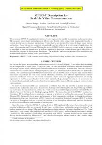
Prokaryotic protein translation is quite well understood in terms of the players involved and an important body of literature exists, providing experimental results that can help create mathematical models. Here a brief overview of prokaryotic translation is presented, so as to understand the system that is to be modeled by this paper.1 . The initiation of translation is summarized in figure2.1. The two main steps are the high affinity bindings of the ribosomal 30s subunit to the 5’ end of a free mRNA strand, followed by the binding of the ribosomal 50s subunit along with the tRNA carrying methionine, placed on the ribosomal A site. Ribosomes are large ribosomal RNA/ ribosomal protein (65%, 35%) complexes, of a length of about 20nm, weighing about 2700kD2 . Due to their size, the ribosomes occlude a certain number of codons on the mRNA when they are bound to it. This is referred to as their Occlusion Distance. Because prokaryotes do not possess a nuclear membrane, DNA is translated into mRNA that quickly becomes bound to ribosomes as the mRNA is churned out from the RNA polymerase. As long as a given length of the 5’ end of the mRNA is accessible (not occluded by a ribosome), another ribosome can bind to the same strand, resulting in a 1D row of ribosomes moving 1 2
Wikipedia: http://en.wikipedia.org/wiki/Prokaryotic translation http://redpoll.pharmacy.ualberta.ca/CCDB/cgi-bin/STAT NEW.cgi
7
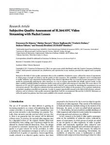
Figure 2.1: The initiation of protein synthesis in prokaryotes, in a condensed c form. Image Richard Wheeler (Zephyris) 2005, from the free licensed media file repository Wikimedia. along the mRNA, which is commonly known as a Polysome. The elongation process involves several steps that are summarized by the model of Zouridis & Hatzimanikatis [20, 21] (See Figure 2.3 ). For the purpose of this work, it is enough to notice that the elongation process revolves around the 1D movement of ribosomes along the length of the mRNA, which each step matching a codon to its anti-codon on the tRNA, and adding an amino acid to the growing protein chain. Each codon that makes up the natural genetic code of most organisms, consists of a triplet of any of the four nucleotides (A,U,C or G), yielding a total of 64 possible nucleotide combinations. Considering that there are 20 amino acids that are digitally coded this way, different codons can code for the same amino-acids. The apparent redundancy (or genetic code degeneracy) confers robustness to protein translation and also adds a new level of transcription regulation [3, 14, 16], through variable codon transcription rates for the same amino-acids, which will be discussed during this work. A table of the natural genetic code is available in the annex (Figure9.1). The termination process occurs when a ribosome encounters a STOP codon while reading the mRNA. This causes the unbinding of the two ribosomal subunits and the liberation of the newly synthesized peptide chain.
8
2.3
Modeling Translation
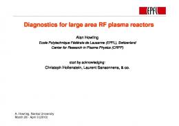
Following is a very brief introduction to modeling in systems biology, in either deterministic or stochastic form. Continuous Deterministic Models For a long time, deterministic models have been the main focus of systems biology. The concept behind these is that a biological system or pathway consists of a series of inputs and outputs that can be expressed in terms of ingoing and outgoing fluxes for each species in the system. These fluxes represent the change in time of the different species in the system, and are expressed by using mass action kinetics, laws that allow to explain the behaviors of solutions in dynamic equillibrium. The flux expressions make up sets of ordinary differential equations (as well as other types) that can then be solved through numerical integration. They offer both quantitative and qualitative insights as to the behavior of the system over time and at steady state. Example: Heinrich-Rappoport Model Heinrich and Rappoport [6] presented a deterministic model of protein translation that takes into account the physical consequence of ribosomes sitting on mRNA by attributing them an occlusion distance L. In their model, by varying the elongation rate KE , the initiation rate KI , and the termination rate KT , they go on to show how ribosomes pile up on an mRNA strand, and how this affects protein production and polysome size. A sample result is shown on figure 2.2. Example: Hermione In a paper by Hermione Zouridis and Vassily Hatzimanikatis [20, 21], a more in-depth deterministic, sequence-specific model is proposed, taking into account most of the known reactions of the elongation process explicitly. This allowed for the elongation rates to be codondependent as well as offering a more accurate model that made fewer assumptions, based on first principles rather than ad-hocassumptions A summary of the model is discussed in figure 2.3. The elegance in the approach lies in considering the ribosomes as molecules at different states (corresponding to different steps in the elongation process), and the development of control parameters to quantify the influence of each state on the system, gaining a better understanding of the limiting steps in the translation process, depending on the parameters used. The conclusions drawn from their studies are as follows (non-exhaustive):
9
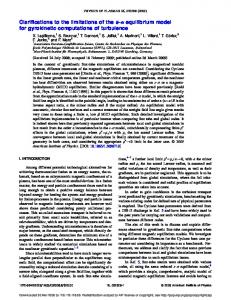
Figure 2.2: Synthesized proteins per minute and mean polysome sizes for αglobin with varying initiation rate (KI )(x axis). Ignore the dashed lines. Values of the curves: (a) 1 mRNA, large ribosome excess (100), KE =43.2min−1 , KT = 6.0min−1 ; (b) KT = 6.0min−1 ; (c) Kw = 90.0min−1 • Increasing polysome sizes lead to increased protein translation rate, which reaches a maximum, and then decreases again, due to overcrowding. • The kinetics are initiation and elongation limited for low polysome sizes and are termination limited for high polysome sizes. • The maximum protein synthesis rate occurs at the polysome size corresponding to the maximum elongation rates for which polysome distributions are still uniform along the length of the mRNA. These points are summarized in figure 2.4, taken from [20]. 10
718 718
that accounts for all the elementar that accounts for all the element mechanism. Specifically, our mode mechanism. Specifically, our mod tary steps involved in the elongat tary steps involved in the elonga along the length of the mRNA. W along theto length of the analysis determine themRNA. effects W analysis to determine the effects and concentrations of the translat and concentrations the transla protein synthesis rate.ofUtilizing ou protein synthesis rate. Utilizing and sensitivity analysis, we investio and synthesis sensitivityproperties analysis, we tein of ainves sin tein synthesis properties of a determine the protein synthesis ras determine the protein synthesis some size and then identify rang some size and then identify which the translation kinetics ran are which the translation kinetics and termination-limited. Additiona and termination-limited. Additio ribosomes are distributed with res ribosomes are distributed with intermediate state and sequence pr intermediateand state and sequence elongation-, termination-limite elongation-, and termination-limi how each elongation cycle element kinetics of elongation a given elongation cycl how each cycle eleme version model. We propose kineticsofofour a given elongation cyc given polysome size depends on t version of our model. We propo tween of elon given ribosomal polysomeoccupancy size depends on states and ribosome distributions w tween ribosomal occupancy of elo sition along the length of the mRNA states and ribosome distributions to polysome self-organization that sition along the length of the mRN maximum levels. to polysome self-organization th maximum levels. METHODS
METHODS steps of the elon Elementary
Elementary stepsphase of the elo The translation elongation is a cycli ribosomes, amino acids, tRNAs, elongation is (Fig. a cyc1 toThe the translation assembly ofelongation polypeptidephase chains ribosomes, acids, tRNAs, elongatio tRNA) bindsamino to Ef-Tu:GTP, forming a te to the assembly polypeptide chains to (Fig ternary complex of then binds reversibly th tRNA) binds to Ef-Tu:GTP, forming a independent manner (Step 1). After findin ternary complex then bindsbinding reversibly reversible codon-dependent (Stepto2 FIGURE 1 (A) The elementary mechanistic steps of the translation independentchanges mannerposition (Step on 1). the After find Ef-Tu:GDP ribosom elongation process. Ribosomal A, P, and E sites indicated on the intermereversible codon-dependent binding (Step 5). In a two-step process, Ef-Ts catalyze re FIGURE 1 (A)Steps The1 and elementary mechanistic steps1, Reversible, of the translation diates between 2 and Steps 9ofand 10.elementary Step codonFigure 2.3: A: Schematic representation the steps of the11Ef-Tu:GDP elongachanges position on thethe ribos and 12). During accommodation, aa-t elongation process. Ribosomal A, P, and E sites independent binding of the ternary complex to theindicated ribosomalon A the site.intermeStep 2, 5). In aand two-step process, catalyze change enters the A siteEf-Ts (Step 6). Trans tion process.diates B: Graphical representation of10. the elongations steps considered Reversible, codon-dependent binding complex to the ribosomal between Steps 1 and 2 and Stepsof9the andternary Step 1, Reversible, codonwhere the peptide chain is transferred from 11 and 12). During accommodation, the a in the Zouridis & Hatzimanikatis model. A site. Stepbinding 3, GTP of hydrolysis. Step 4, Ef-Tu:GDP position change on the independent the ternary complex to the ribosomal A site. Step 2, tRNA, resulting in the A elongation of the p change and enters site (Step 6). Tran ribosome. codon-dependent Step 5, Ef-Tu:GDPbinding release.of Step aa-tRNA accommodation. Step Reversible, the6, ternary complex to the ribosomal acid. Reversible binding of is Ef-G:GTP (Step where the peptide chain transferred fr Transpeptidation. Step 8, Reversible binding of Ef-G:GTP. 9, A7,site. Step 3, GTP hydrolysis. Step 4, Ef-Tu:GDP position changeStep on the 9). During translocation P site tRNA and tRNA, resulting in thethe elongation of the While providing very valuable information on the Translocation. 10, E siterelease. tRNA release. 11 and 12,description Ef-Ts catalyzed ribosome. Step 5,Step Ef-Tu:GDP Step 6,Steps aa-tRNA accommodation. Stepof the transribosome and the A site tRNA and codon(St m acid. Reversible binding of Ef-G:GTP Ef-Tu:GTP. 13, Ef-Tu:GTP binding to the aa-tRNA. 7,regeneration Transpeptidation. Step 8, Step Reversible binding of Ef-G:GTP. Step of 9, noise lational machinery, theof Z-H model cannot capture the effects since complex moving toward the 39 end of the m 9). During translocation the P site tRNA a Steps 14 and 15, of Ef-G:GTP. (B) A representation StepRegeneration 10, site tRNA release.So Steps 11graphical and 12, Ef-Ts catalyzed inribosome the E site is the released the processesTranslocation. are modeled as Econtinuous. information about the stochastic and A sitealong tRNAwith andEf-G:G codon of the elementary elongation steps of the translation elongation process with regeneration of Ef-Tu:GTP. Step 13, Ef-Tu:GTP binding to the aa-tRNA. recycled a two-step process (Steps 14the an complexinmoving toward the 39 end of nomenclature from the model of formulation explained in therepresentation text. Fluxes Steps 14 and 15, Regeneration Ef-G:GTP.as(B) A graphical ð1Þ ð#1Þ in the E site is released along with Ef-G: and Vij;n;r elongation represent steps reversible, binding of with the ij;n;relementary ofVthe of the codon-independent translation ð2Þ elongation process ð#2Þ recycled in a two-step process (Steps 14 Vij;n;rtext. represent ternary complex themodel ribosomal A site. Fluxes Vij;n;r and nomenclature fromtothe formulation as explained in the Fluxes Model formulation 11 ð1Þ ð#1Þ reversible, codon-dependent binding of the ternary complex to the ribosomal represent reversible, codon-independent binding of the Vij;n;r and Vij;n;r ð3Þ ð4Þ ð5Þ ð2Þ GTP hydrolysis. Fluxes Vij;n;rand andVVð#2Þ A site.complex Flux Vij;n;rtorepresents We have employed the following assump ij;n;r represent ternary the ribosomal A site. Fluxes Vij;n;r ij;n;r represent Model formulation Ef-Tu:GDP position change on the ribosome and Ef-Tu:GDP release, mathematical model for the elongation cycl reversible, codon-dependent binding of the ternary complex to the ribosomal ð6Þ ð7Þ Fluxes Vij;n;r respectively.ð3ÞFlux Vij;n;r represents aa-tRNA accommodation. ð4Þ ð5Þ the elementary steps of the elongation cyc represents GTP hydrolysis. Fluxes V and V represent A site. Flux V We have employed the following assum ð#7Þ ij;n;r ð8Þij;n;r and Vij;n;r represent reversible binding of Ef-G:GTP.ij;n;r Flux Vij;n;r represents model formulation is included in Fig. 1 B. Ef-Tu:GDP position change on ð9Þ the ribosome and Ef-Tu:GDP release, mathematical model for the elongation cy ribosomal translocation. Flux ðV Þ represents E site tRNA release. The ð6Þ ð7Þ aa-tRNA accommodation. Fluxes Vij;n;r respectively. Flux Vij;n;r representsij;n;r the elementary steps of the elongation c intermediate elongation cycle states that occur before and after ð#7Þ ð8Þ transpeptiand Vij;n;r represent reversible binding of Ef-G:GTP. Flux Vij;n;r represents ð7Þ model formulation is included in Fig. 1 B elongation cycle is ready to begin with the dation (Step 7, panel A) are considered to be one state in our model ðS Þ. ð9Þ The ribosomal translocation. Flux ðVij;n;r Þ represents E siteð9ÞtRNA release.ij;n;r After release of the tRNA in the ribosomal E site ðV Þ, the subsequent codon n11.
726
FIGURE 6 Scaled effective codon sequence position under elongation-limited (r ¼ 0.95, da dotted line) conditions.
the characteristic effectiv elongation-limited kineti effective elongation cons times the characteristic eff protein synthesis rates are termination-limited condi stants are approximately e effective elongation rate ribosome length apart du length of the mRNA, wh gation rate constants var FIGURE 5 Relationships between translation properties and polysome much Figure 2.4: Protein production rates with respect to ribosomal density ρ. A: as the characteristic size using the MG-HR model. (A) Specific protein production rate as a funcIn the reduced model the Plot showing maximumsize. production rate. B: Control parameters for Initiation tion of polysome (B) Initiation (solid vline), elongation (dashed line), v v theasdenominator of the ex CKI , Elongation, CKE(dotted , and line) Termination CKT , and their relative influences and termination control coefficients as functions of polysome eff polysome sizes increase. tion rate constant, kE;n;r size. increases as Un,r decrease some size, ribosomal crow behavioreffective of the system cannot recovered. elongation ratebeconstant magnitudes that are speeff is appro Un,r ! 1 and kE;n;r cific to different polysome sizes. These results are used to effective elongation rate investigate how self-organization of bound ribosomes with creases, ribosomal crowd respect to the elongation cycle state and position occupancy eff decreases causing kE;n;r to affects the relationship between translational behavior and ribosomal crowding on th 12 polysome size. eff to approach causing kE;n;r rate constant, k8. Hence, a elongation rate constants Effective elongation rate constants and length apart are approxim polysome size protein synthesis rate oc sponding to the set of effe To investigate differences between the results of the ZH
Discrete Stochastic Models Stopping for a moment to consider the nature of the systems under study, it can be shown that under certain conditions, modeling in continuous form is not sufficient [8]. Deterministic models are acceptable when faced with very large numbers of molecules, so that the way their fluxes are expressed approximate the molecular fluxes happening at the thermodynamic limit. In practice, a system is usually considered to be at the thermodynamic limit when its molecule numbers are close to the Avogadro number(6.022.1023 Molecules). Below this value, deterministic modeling is not sufficient because the discrete nature of the system generates stochastic behaviors. Cellular processes are confined to a small volume (that of the cell) and to small molecule numbers, so many of them operate under the thermodynamical limit. With about 4’000 mRNAs and 18’000 Ribosomes, a typical E.coli cell cannot be modeled in a deterministic way if emergent behavior caused by stochastic processes wants to be studied . In the case of protein translation, the discrete nature of the states of the molecules, such as the availabilities of free mRNAs for ribosome binding or the one-codon-at-a-time movement of the ribosome along an mRNA strand, require a discrete ‘per step’ view that reflects the finite nature of the system, also called a jump Markov Process. To remedy this with the help of computers, methods for modeling discrete systems have been developed, and take many forms, such as Markov Models, Petri Nets, and Kinetic Monte Carlo Monte Carlo methods rely on random number generators to simulate the non-deterministic nature of the systems being modeled. (For a good introduction, the book ”Stochastic Modelling for Systems Biology” by Darren J. Wilkinson is suggested). The difference between deterministic models and stochastic models, mathematically speaking, is that rather than considering the fluxes of molecules going from a given state or species to another, these models deal with the probabilities of these events taking place inside a certain volume with certain molecule numbers (not concentrations). One ends up with a linear system of differential probability equations, called the chemical master equation (2.1).
13
�
�
�
�
~ t + dt|X ~ 0 ; t0 = P X; ~ t|X ~ 0 ; t0 1 − P X;
M X j=1
aj dt+
M X
�
�
~ − ~vj ; t|X ~ 0 ; t0 dt P X
j=1
(2.1)� ~ is the state vector of the system with P X; ~ t|X ~ 0 ; t0 In this expression, X ~ at time t, given that the state was X ~0 the probability that the state is X at time t0 . The first expression in the right-hand side sum then represents the probability that no reaction takes place in the interval t + dt, and the second expression represents the probability of there being a reaction ~v so ~ − ~vj at time t. M is the number of reactions that the system was at X in the system and aj = cj .hj is the propensity of reaction j, that is the probability that reaction j will occur within t + dt in the volume considered. cj is the mesoscopic reaction rate constant of reaction j and hj is the number of possible combinations of the reacting molecules of reaction j. One cannot solve the chemical master equation explicitly for anything but the smallest systems, as it grows combinatorially. What can be done using Monte Carlo methods is to recover a realization of the chemical master equa~ tion. � By taking � the data of many runs into X that follow the constraints of ~ ~ P X; t|X0 ; t0 , it is possible to infer the complete state-space of the system. �
Example: Mitarai Paper This Masters project started by replicating the algorithm developed by Mitarai et al. [15], which uses a Monte Carlo simulation with a constant time step ∆t. At each step, the probability of a ribosome binding to mRNA is calculated as Ksf ∆t, the probability of bound ribosomes to move as KE (codon)∆t, the probability of a ribosome at position L to unbind from the mRNA as KT ∆t. With Ksf , KE (codon) and KT the initiation, codon-dependent elongation and termination rate constants. Figure 2.3 offers a schematic representation of the different steps involved in their model. This paper also deals with a further aspect of protein translation which was mRNA rates of birth and decay, which will not be included here. The model was tested against experimental data of recombinant protein production using the LacZ plasmid and a modified construct, where ”slow” codons were added. The output they observed was protein production using radioactively labeled amino-acids. By looking at the accumulated radioactivity in lacZ operon variants and using their Monte Carlo agorithm to replicate the radioactivity measure14
Using this model of translation reproduce the in vivo experiment for radioactivity in a model protein.2 Th performed as follows: At time t = 0, mRNAs being translated in steady st a 10-s pulse of radioactive 35S-methi is stopped by adding a large exce Results methionine to the culture. After this are taken at 10-s intervals and the rad completed protein is determined. F Description of the model of translation kinetics schematic incorporation curve. Th ments, they able tothe show that the presence of ribosomalmRNA queueing duethe ordinate axis illustr along First,were we model basic dynamics of translation. 35 to variable elongation rates was the most likely factor explaining data (Figure after the S-Met pulse and chase, Figure 1 depicts ribosomes that translate an mRNA. 2.6). Translation starts by binding a 30S ribosomal that were close to terminating at the , provided that subunit to codon 1 with the rate K Through their discussion, show that as fully deterministicwill or contribute a uniform radioactivity to the f As time to progresses and more sam binding site accessible, which requires were that no codon the distribution foristhe stochastic mechanism not sufficient demore and more radioactivity will ac ribosome is within the occluding distance, d, from scribe the model, explaining that the variable codon elongation rate confinished peptide. When the first r the binding site. The ribosome stays at codon 1 for a stants, though creating bottlenecks close to slow codons, also helped regulate mRNA at the time of the pulse time, τ, to assemble the translating 70S ribosome. translation through careful codon usage. experimental data on lacZ translation with and without slow inserts in a model. We now can analyze how codon usage and mRNA stability may be used to influence speed, expression yield, and metabolic cost associated to protein production.
Fig. 1. Visualiz eled translation Ribosomes move codon on an mR tion rates that dep Each ribosome oc 11 subsequent co quent ribosomes a rate given by K forming the 70S i is usually set to middle bar indic Figure 2.5: Schematic representation of Monte Carlo model that was used in of methionine re the Mitarai paper. R1 , ..., Rx are the different codon-specific rates. Ks, the The lower panel bution of the f Initiation rate and Kt the termination rate. codons (yellow), codons (blue), and the slowly translated C codons (red) in the 1027 codons of the parental lacZ gene in ribosome reaches the stop codon, it is terminated with the nonlimiting rate constant of 2/s.
Gillespie’s Algorithms
The paper by Mitarai et al. is an elegant approach at modelling protein translation in a stochastic form, but has certain limitations that this work aims to overcome. • Ribosomes are considered to be in excess, thus ribosomal concentrations play no role in the model. However, in E.coli , the concentration of ribosomes translates to about 18’000 per cell. If one considers 1000 mRNAs, that means that there are about 18 ribosomes available per mRNA on average. The similarity of scale demands for ribosomes to be considered explicitely.3 • The framework is a fixed time step Monte Carlo which does not capture the physical properties of the system, which consists of chemical 3
E.coli Stats: http://redpoll.pharmacy.ualberta.ca/CCDB/cgi-bin/STAT NEW.cgi
15
the mRNA. Already at 30 translations per mRNA, the stochastic effects have increased the average translation time by 5% compared to an mRNA that was only translated once. Figure 5a also shows that a stable mRNA would be translated 1.7% slower than the present lacZ mRNA translated on average 30 times. This suggested to us that bacteria might have evolved unstable mRNAs as yet another way to
waste their time by collisio
Fig. 5. (a) Average translati
4. time Space–time of ribosome as simulated Figure 2.6: Fig. Space plot of plot ribosome traffictraffic for the LacZ Operon.cost Forofthetranslation as a functio translations, with parameters from Fig. 3b. Each red dotted line refers wild type LacZ (a) and for the LacZ gene with an insert of slow codons at the p, per mRNA. The by ATP molecules needed to ad to the movement of a single ribosome along the DNA. end of theWhen sequence. For figures a,b and we see how translation machinery such tha ribosomes slow down, for c, example, whenindividual queues ribosomes (red lines)are move along theone mRNA over timedensity for 30 proteins being translated. tion is fixed to the same valu developing, sees increased of ribosomes. Figure d shows how aofqueue can develop on an mRNA. Methods). The solid curve is the Translation (a) pMAS23, (b) pMAS24GAG, and (c and
function of p. The three dashed d) pMAS48GAG. In (a), (b), and (c), we translate mRNAs cost, including an mRNA proce exactly 30 times. In (d), we show how a queue develops reactions occurring due to molecular collisions 280which million ATPs per cell, respe on a stable mRNA with the long, slow insert.in a given volume
carries with it some implications and should therefore have a framework that encompasses this physical system. • Consider the 4’000 mRNAs in a typical E.coli cell. They are not all the same mRNAs and code for different genes at different rates. The developed algorithm should allow the study of mRNA competition for a shared pool of ribosomes among different species. • Due to the microscopic nature of the system, noise is of importance. LiKE mentionned above, the study of noise propagation should be considered. Namely, how does initiation noise (Collisions of molecules in 3 16
dimensions, ribosomes binding to mRNA) relate to termination noise (unbinding of a ribosome after passing through a 1D system) and how would noise propagate in the system. In 1977, Daniel T. Gillespie [2] proposed a stochastic simulation algorithm (SSA) that offered a framework in which the physical nature of the system was taken into consideration as well as an easy to implement method that served as the backbone for the rest of the algorithm to be written into. A quick summary of the algorithm is presented in figure 2.7. How It Works (Direct Method) Gillespie’s analysis shows that in a well-mixed discrete system driven by many non-reacting elastic collisions of molecules that bring reacting species together, the probability of two molecules colliding in an infinitesimal time can be rigorously calculated. He then proposed to break down the simulation into single reaction steps, where at each step the questions“When will the next reaction take place?” and “What kind of reaction will it be?” are asked. Using two random numbers, one exponentially distributed that gives the time to the next reaction, and the second uniformly disctributed that gives the type of reaction that will take place, Gillespie showed that it yielded an unbiased walk in the probability space of the system. This is called Gillespie’s ”Direct Method”. Variants of this algorithm exist, such as the Next Reaction Method and First Reaction Method, and although they were not used in this work, they could be easily extended for the use of this algorithm.
17
actions
MOLECULE
2341 1
'0
'Input valuer for e" ["=I,. ..,hi).
for
.input initial
xi
[