use the similarity between the desired and undesired signal subspaces obtained from the sample spatial PSD matrices, as an indicator of the achievable spatial ...
ITG-Fachbericht 252: Speech Communication, 24. – 26. September 2014 in Erlangen
A subspace-based perspective on spatial filtering performance with distributed and co-located microphone arrays Maja Taseska, Emanuël A. P. Habets International Audio Laboratories Erlangen1 Am Wolfsmantel 33, 91058 Erlangen, Germany {maja.taseska, emanuel.habets}@audiolabs-erlangen.de
Abstract
In this work, we investigate whether the distance between the desired and undesired signals subspaces can be used as an indicator of the achievable spatial filtering performance, without specific assumptions on the employed filter. The desired and undesired signal subspaces are obtained from the corresponding sample spatial PSD matrices and the subspace (dis)similarity is expressed as a distance function on the Grassmann manifold [9]. A distance function is computed using the principal angles between the subspaces. We investigate the subspace distances for different reverberation levels and different relative sourcearray positions. Particularly, we compare distributed arrays and arrays with co-located microphones, and show that there is a relation between the subspace distances and the achievable interference reduction. The spatial filtering in the evaluation was performed using an MVDR filter. The rest of the paper is organized as follows: in Section 2 the signal model is presented. In Section 3, the concept of a subspace distance is reviewed and its application to speech signals is proposed. Experimental results investigating the subspace distance and its effect on spatial filtering for different reverberation times and array configurations are presented in Section 4. Section 5 concludes the paper.
Commonly used data-dependent spatial filters depend on the acoustic transfer functions and the power spectral density (PSD) matrices of the desired and the undesired signals. Assuming a low-rank model of the spatial PSD matrix of the signals, and a particular spatial filter, the performance in terms of a given objective measure can often be described analytically. In this paper, we propose to use the similarity between the desired and undesired signal subspaces obtained from the sample spatial PSD matrices, as an indicator of the achievable spatial filtering performance. The subspace similarity is expressed as a distance function on the Grassmann manifold, computed using the principal angles between the subspaces. Particularly, subspace distances and spatial filtering performance are compared when using distributed arrays and co-located microphones. Experimental results demonstrate the relation between these two different measures for different array configurations and reverberation levels.
1 Introduction Many multichannel speech enhancement algorithms are derived using a low-rank linear model for the spatial PSD matrix of a speech signal. Based on such a model, the vectors containing the speech signal at different microphones lie in a low dimensional subspace, which depends on the acoustic transfer functions (ATFs) from the source to the microphones. The low dimensionality of the speech signal subspace is exploited, for instance, in speech enhancement, by decomposing the received microphone signals into a desired signal subspace and an undesired signal subspace [1]. This idea also forms the basis of some of the most widely used parameter estimation algorithms such as MUSIC and ESPRIT [2, 3]. In the presence of undesired sources, the low dimensionality of the signals allows for spatial filtering that can completely suppress the undesired source signal without distorting the desired signal, if the signals span different non-overlapping subspaces. Given the rank-one spatial PSD model, and a particular spatial filter, the performance in terms of a given objective measure can often be described analytically. For instance, an evaluation of the tradeoff between dereverberation and noise reduction of the minimum variance distortionless response (MVDR) filter was presented in [4], whereas the authors in [5] examine the MVDR filter for different noise fields and source incidence angles. The average output signal-to-noise ratio (SNR) of the Wiener filter for a given array configuration was derived in [6], while the performance of filters with a generalized sidelobe canceller structure has been investigated in [7, 8].
2 Signal model We consider a mixture of a desired signal and an undesired signal received at the M microphones of a traditional array with co-located microphones, or at the microphones of multiple distributed arrays. The signals are transformed to the time-frequency (TF) domain by a short-time Fourier transform (STFT), such that the complex spectral coefficients of the microphone signal vector y are given by y(n, k) = xd (n, k) + xi (n, k) + v(n, k),
where xd , xi , and v denote the desired signal, the undesired signal, and the background noise at the microphones, and n and k are the time and frequency indices, respectively. In the case of point-like sources and sufficiently long STFT frames that capture the main part of the room impulse responses (RIRs) between the sources and the microphones, the vectors xd and xi lie in a lower dimensional linear subspace of the M -dimensional complex vector space CM [10]. The subspaces spanned by the desired and undesired signals can be obtained from the PSD matrices of the random vectors xd and xi , given by � � Φ d (n, k) = E xd (n, k)xH (2a) d (n, k) , � � H Φ i (n, k) = E xi (n, k)xi (n, k) . (2b) Many data-dependent spatial filters that extract the desired signal while reducing the noise and the undesired signals are computed using estimates of the PSD matrices Φ d and
1A
joint institution of the University Erlangen-Nuremberg and Fraunhofer IIS, Germany
ISBN 978-3-8007-3640-9
(1)
1
© VDE VERLAG GMBH  Berlin  Offenbach
ITG-Fachbericht 252: Speech Communication, 24. – 26. September 2014 in Erlangen
Φ i . For the purpose of this investigation, we assume that the signals xd and xi are available, and the respective PSD matrices are computed for each frequency by a recursive averaging over time frames, as commonly done in practice. In this manner, the PSD matrices at a time frame n are obtained according to Φ d (n) = α Φ d (n − 1) + (1 − α) xd (n)xH d (n),
(3a)
Φ i (n) = α Φ i (n − 1) + (1 − α)
(3b)
xi (n)xH i (n),
tion problem, the principal angles can be efficiently computed using the singular value decomposition (SVD), as proposed in [16]. The principal angles between A and B can be computed by the following steps: (i) Compute orthonormal bases U = [ u1 | · · · | ud ] and V = [ v1 | · · · | vd ] for A and B. (ii) Compute the matrix G(U , V ), where the entry at the i-th row and j-th column is given by |�ui , vj �|. (iii) Compute the SVD G(U , V ) = Y Σ Z H . (iv) The principal angles are obtained as
where α is an averaging constant, and the frequency index has been omitted for brevity. In the following we introduce the concept of subspace distances used to analyze the (dis)similarity between the subspaces spanned by Φ d and Φ i and its implications on spatial filtering performance.
Σ = diag[cos(θ1 ), · · · , cos(θd )].
Given the principal angles θ = [θ1 ,· · · ,θd ], the geodesic distance between A and B is given by Dg (A, B) = �θ�2, where � · �2 denotes the Euclidean norm. Besides the geodesic distance on the Grassmann manifold, commonly used distance measures computed as a function of the principal angles include the projection metric, minimum correlation metric, Procrustes metric, etc. [11] In this work, we use the projection metric, which is computed from the principal angles as follows � �1/2
3 Computing subspace distances The subspaces spanned by the desired and the undesired signal vectors xd (n, k) and xi (n, k) can be interpreted as points on the Grassmann manifold. The Grassmann manifold has a Riemannian structure that allows the computation of distances between the points on the manifold. In the following, we discuss distance measures on the Grassmann manifold, and propose to use them for characterizing the subspace similarity in the context of speech processing.
Dp (A, B) =
The set GC (d, M ) of all d-dimensional linear subspaces of the M -dimensional complex vector space CM is a smooth manifold of dimension d×(M − d), known as the complex Grassmann manifold [9]. The elements of GC (d, M ) consist of all full-rank matrices A ∈ CM ×d . Two elements A, B ∈ GC (d, M ) are equivalent, if and only if they span the same subspace, i.e., there exists a unitary matrix Q such that A = BQ. The Grassmann manifold is used in a variety of signal processing, optimizaton, and machine learning applications (see [11, 12] and references therein). The Grassmann manifold has a Riemannian structure which allows to compute distances between points, hence a dissimilarity between two subspaces of dimension d can be viewed as a distance function on the complex Grassmann manifold. For instance, the geodesic distance between two subspaces in GC (d, M ) can be used as a distance function which is related to the principal angles between the subspaces [13, 14]. Besides the geodesic distance, different distance metrics can be computed in terms of the principal angles, as described next.
|�u, v�|,
subject to �u, ui � = �v, vi � = 0, for i = 1, . . . , k − 1, �u� = �v� = 1,
.
(6)
4 Experimental results To investigate the distance between the subspaces spanned by the PSD matrices Φ d and Φ i at each frequency and its effect on spatial filtering, we simulated signals corresponding to the scenario shown in Fig. 1. In order to have a desired and undesired signal energy at each frequency bin for the distance investigation, white noise signals were convolved with simulated RIRs [17], whereas for the spatial filtering clean speech signals were convolved with the same RIRs. We investigated the following array configurations (see Fig. 1 for numbering of the arrays): (i) One array
(4a)
(4b) (4c)
where � · � and �·� denote the Euclidean norm and the inner product, respectively. Rather than solving the optimiza-
ISBN 978-3-8007-3640-9
k=1
The steps (i)-(iv) from Section 3.2 can be performed for the spatial PSD matrices of the desired and the undesired speech signal, i.e., A = Φ d and B = Φ i . If the rank-one assumption holds, the subspace distance depends only on the Hermitian angle between the ATF vectors of the desired and the undesired source, which is equivalent to the principal angle for one-dimensional subspaces. However, at high reverberation levels the rank of the sample PSD matrices and their corresponding subspaces increases due to the limited support of the STFT window. The correct subspace dimension can be chosen for instance by counting the significant eigenvalues of Φ d and Φ i . Note that the desired and undesired signal subspaces might have different dimensions. In such cases, the two subspaces are not represented as points on a Grassmann manifold with a given dimension. Nevertheless, the principal angles can be computed as shown in Section 3.2 between subspaces with different dimensions as well, and the projection metric still represents a valid distance metric between the subspaces.
The extension of the concept of principal angles to complexvalued vector spaces was discussed in [15].The d principal angles θ1 ,. . .,θd between subspaces A ∈ GC (d, M ) and B ∈ GC (d, M ) are recursively defined by the following optimization problem max
∑ sin2 (θk )
3.3 Application to speech processing
3.2 Principal angles and subspace distances
u∈span(A),v ∈span(B )
d
Given the matrices PA and PB , which perform orthogonal projection onto the subspaces spanned by A and B, respectively, the projection metric can be also computed by Dp (A, B) = 21/2 �PA − PB �F , where � · �F denotes the Frobenious norm of a matrix.
3.1 Complex Grassmann manifold
cos(θk ) =
(5)
2
© VDE VERLAG GMBH  Berlin  Offenbach
ITG-Fachbericht 252: Speech Communication, 24. – 26. September 2014 in Erlangen
��
�� � � � ��
��
bands, (0, 1.5] kHz and (1.5, 8] kHz, as well as fullband. The ΔDSIR values for the different array configurations and reverberation levels are shown in Figure 3. The input DSIR was 1.3 dB and -0.5 dB at Array1, and 2.6 dB and 0.5 dB at Array2, for the low and high frequencies, respectively. When using multiple arrays, the reference microphone for the filtering was always chosen from Array1. To ensure that the undesired signal PSD matrix is invertible for the MVDR implementation, we added white Gaussian noise to the microphone signals with a signal-to-noise ratio of 50 dB. However, to compute the performance measures, only the speech signals were considered. Relating the DSIR improvement and the subspace distance results discussed in Section 4.1, we can summarize the following observations (i) The advantage of using multiple arrays over a single array increases with increasing T60 , as shown in Figure 3(a) for the lower frequency band. Similarly, the difference in subspace distances was most significant in this frequency band as well. (ii) The values of ΔDSIR for the higher frequency band shown in Fig 3(b), are similar for all array configurations, and higher than the values for the lower frequency band. The subspace distances were likewise high for all array configurations. (iii) The performance of Array2 is consistently the lowest. In contrast to the other array configurations, where the best performance is achieved in non-echoic environment, the performance of Array2 is the worst in this case, and increases with increasing T60 . The same trend was observed for the subspace distances related to Array2. The fullband SD index νsd is shown in Figure 5. The oracle PSD matrix estimates and the distortionless constraint of the MVDR filter ensure that the SD index is very low in all cases, with a tendency to increase at higher T60 .
� �������
����� �
��
�� � � � � � � �
�
� ������� ����� � ����
Figure 1: Scenario used in the evaluation. Shoebox room with dimensions 6×5×3 m. with six microphones (Array1), (ii) one array with six microphones, with respect to which the desired and undesired signal have the same direction-of-arrival (Array2), (iii) two arrays, (Array1 and Array2) with three microphones each, and (iv) three arrays with two microphones each. The inter-microphone distance at each array was 4 cm. Note that for all configurations, the total number of microphones is six. The sampling frequency was 16 kHz and the STFT frame length was 64 ms with 50% overlap.
4.1 Results: Subspace distances The geodesic distance Dg and the projection distance Dp between the desired and the undesired signal subspaces was computed on the 1-D and 2-D Grassmann manifolds. The two distance measures showed similar trends across frequency for all array configurations. For further evaluation, we chose to use the projection distance Dp , in view of the fact that this distance can be measured between subspaces of different dimensions as well, as mentioned in Section 3.3. The results for different reverberation times are shown in Fig. 2. Comparing Array1 and Array2, it can be noted that the subspace distance strongly depends on the relative array-source position. Particularly, in a nonechoic environment, shown in Figure 2(a), the distance is very low if the direction of arrivals (DOAs) of the sources are equal with respect to the array. However, the distances for Array2 increase with increasing reverberation time T60 due to the room reflections which depend on the source position. Due to the larger spatial coverage of distributed arrays, it is less likely to have source locations that cause high subspace overlap, as for Array2. Most significant difference between a single array and multiple arrays is observed at frequencies up to 1.5 kHz, especially for higher values of T60 . Note that for high T60 and fixed STFT window size, the subspace dimension increases. As there were two significant eigenvalues in the PSD matrices of the desired and undesired signals, we computed the distance between 2-D subspaces. The results for T60 =0.6 s, shown in Figure 4, more clearly indicate the advantage of using multiple arrays, particularly at frequencies up to 2 kHz.
5 Conclusions Distance on the complex Grassmann manifold between the subspaces spanned by the power spectral density matrices of a desired and an undesired signal was proposed as an indicator of spatial filtering performance. The advantage of distributed arrays over co-located microphones was interpreted from the subspace distance perspective, where especially at higher reverberation times and frequencies up to 1.5 kHz, distributed arrays outperform co-located microphones. The results from the subspace distance investigation were corroborated by a spatial filtering example, where a desired speech signal was extracted using an MVDR filter. It was shown that distributed arrays outperform in all cases, especially at frequencies where the subspace distances are significantly larger as well. Future work includes further investigation of the relation between subspace distance and spatial filtering performance.
References
4.2 Results: Spatial filtering
[1] Y. Ephraim and H. L. Van Trees, “A signal subspace approach for speech enhancement,” IEEE Trans. Speech Audio Process., vol. 3, pp. 251–266, July 1995. [2] R. O. Schmidt, “Multiple emitter location and signal parameter estimation,” IEEE Trans. Antennas Propag., vol. 34, no. 3, pp. 276–280, 1986. [3] R. Roy and T. Kailath, “ESPRIT - estimation of signal parameters via rotational invariance techniques,” IEEE Trans.
An MVDR filter was applied to extract a desired talker and reduce an interfering talker, in the scenario in Figure 1. The performance was evaluated in terms of segmental desired signal to interference ratio (DSIR) improvement ΔDSIR and segmental speech distortion (SD) index νsd [18], where νsd ∈ [0, 1], with 0 indicating no distortion. The value of ΔDSIR was computed separately for two frequency
ISBN 978-3-8007-3640-9
3
© VDE VERLAG GMBH  Berlin  Offenbach
1 0.8 0.6
Arr 1 Arr 2
0.4
Arr 1,2,3 Arr 1,2
0.2 0 0
2
4
6
Frequency (kHz)
Subspace distance Dp
Subspace distance Dp
Subspace distance Dp
ITG-Fachbericht 252: Speech Communication, 24. – 26. September 2014 in Erlangen
1 0.8 0.6
Arr 1 Arr 2
0.4
Arr 1,2,3 Arr 1,2
0.2 0 0
8
2
4
1 0.8 0.6
Arr 2 Arr 1,2,3 Arr 1,2
0.2
6
0 0
8
Frequency (kHz)
(b) T60 = 0.2 s
(a) Anechoic
Arr 1
0.4
2
4
6
8
Frequency (kHz)
(c) T60 = 0.6 s
Figure 2: Subspace distances computed on the 1D Grassmann manifold for different reverberation levels. 20
20
Arr 1 Arr 2 Arr 1,2,3 Arr 1,2
ΔDSIR
10
10
5
10
5
0 0
0.2
0.4
T60 [sec]
0.6
0.8
5
0 0
(a) Frequency band 0-1.5 kHz
Arr 1 Arr 2 Arr 1,2,3 Arr 1,2
15
ΔDSIR
15
ΔDSIR
15
20
Arr 1 Arr 2 Arr 1,2,3 Arr 1,2
0.2
0.4
T60 [sec]
0.6
0.8
0 0
(b) Frequency band 1.5-8 kHz
0.2
0.4
0.6
T60 [sec]
0.8
(c) Fullband
0.08
1.5
0.06
1
Arr 1 Arr 2 Arr 1,2,3 Arr 1,2
0.5
0 0
νsd
Subspace distance Dp
Figure 3: Desired signal-to-interference ratio improvement obtained by an MVDR filter.
0.04
Arr 1 Arr 2 Arr 1,2,3 Arr 1,2
0.02
2
4
6
0 0
8
Frequency (kHz)
0.2
0.4
T60 [sec]
0.6
0.8
Figure 4: Subspace distance on the 2D Grassmann manifold for T60 = 0.6 s.
Figure 5: Desired speech signal distortion after applying an MVDR filter.
Acoust., Speech, Signal Process., vol. 37, pp. 984–995, 1989. E. A. P. Habets, J. Benesty, I. Cohen, S. Gannot, and J. Dmochowski, “New insights into the MVDR beamformer in room acoustics,” IEEE Trans. Audio, Speech, Lang. Process., vol. 18, pp. 158–170, Jan. 2010. C. Pan, J. Chen, and J. Benesty, “Performance study of the MVDR beamformer as a function of the source incidence angle,” IEEE Trans. Audio, Speech, Lang. Process., vol. 22, no. 1, pp. 67–79, 2014. T. C. Lawin-Ore and S. Doclo, “Average output SNR of the multichannel Wiener filter using statistical room acoustics,” in Proc. IEEE Workshop on Applications of Signal Processing to Audio and Acoustics (WASPAA), (New Paltz, NY), 2013. J. Bitzer, K. Simmer, and K.-D. Kammeyer, “Theoretical noise reduction limits of the generalized sidelobe canceller for speech enhancement,” in Proc. IEEE Intl. Conf. on Acoustics, Speech and Signal Processing (ICASSP), vol. 5, pp. 2965–2968, Mar. 1999. G. Reuven, S. Gannot, and I. Cohen, “Performance analysis of the dual source transfer-function generalized sidelobe canceller,” Speech Communication, vol. 49, pp. 602–622, Aug. 2007. S. Kobayashi and K. Nomizu, Foundations of differential
geometry, vol. 2. New York: Interscience, 1969. [10] Y. Avargel and I. Cohen, “On multiplicative transfer function approximation in the short-time Fourier transform domain,” IEEE Signal Processing Letters, vol. 14, no. 5, pp. 337–340, 2007. [11] J. Hamm, Subspace-based learning with Grassmann kernels. PhD thesis, University of Pennsylvania, 2008. [12] J. H. Manton, “On the role of differential geometry in signal processing,” in Proc. IEEE Intl. Conf. on Acoustics, Speech and Signal Processing (ICASSP), 2005. [13] G. H. Golub and C. F. van Loan, Matrix Computations. MD: John Hopkins University Press, Balimore, third ed., 1996. [14] Y.-C. Wong, “Differential geometry of Grassmann manifolds,” in Proc of the Nat. Acad. of Sci., vol. 57, pp. 589– 594, 1967. [15] A. Galántai and C. J. Hegedüs, “Jordan’s principal angles in complex vector spaces,” Numer. Linear Algebra Appl., vol. 13, pp. 589–598, 2006. [16] A. Björck and G. Golub, “Numerical methods for computing angles between linear subspaces,” Mathematics of Computation, vol. 27, pp. 579–594, 1973. [17] E. A. P. Habets, “Room impulse response generator,” tech. rep., Technische Universiteit Eindhoven, 2006. [18] J. Benesty, J. Chen, and Y. Huang, Microphone Array Signal Processing. Berlin, Germany: Springer-Verlag, 2008.
[4]
[5]
[6]
[7]
[8]
[9]
ISBN 978-3-8007-3640-9
4
© VDE VERLAG GMBH  Berlin  Offenbach