A Symbolic-Numeric Method for Solving Boundary Value Problems of

A Symbolic-Numeric Method for Solving Boundary Value Problems of Kirchhoff Rods Liu Shu and Andreas Weber Institut f¨ ur Informatik II, Universit¨ at Bonn, R¨ omerstr. 164, Bonn, Germany {liushu, weber}@cs.uni-bonn.de

Abstract. We study solution methods for boundary value problems associated with the static Kirchhoff rod equations. Using the well known Kirchhoff kinetic analogy between the equations describing the spinning top in a gravity field and spatial rods, the static Kirchhoff rod equations can be fully integrated. We first give an explicit form of a general solution of the static Kirchhoff equations in parametric form that is easy to use. Then by combining the explicit solution with a minimization scheme, we develop a unified method to match the parameters and integration constants needed by the explicit solutions and given boundary conditions. The method presented in the paper can be adapted to a variety of boundary conditions. We detail our method on two commonly used boundary conditions.

1

Introduction

The study of deformations in elastic rods can be applied in several fields. Examples of slender structures in structural engineering are submarine cables or tower cables [1]; in biology elastic rods are often used to study supercoiling and other mechanical behaviors of DNA strands [2,3,4,5]. And in daily life we often see string objects or filaments, like telephone cords, willow branches, climbing plants and human or animals hair [6]. Based on Newton’s second law, the Kirchhoff rod model provides a theoretical frame describing the static and dynamic behaviors of elastic rods [7,8]. The Kirchhoff model holds for small curvatures of rods, but Kirchhoff rods can undergo large changes of shape [9]. In particular, for the static case, all dependent variables appearing in the equations are only functions of one spatial variable, such as arc length of rods. Thus the static Kirchhoff equations are a set of ordinary differential equations. Numeric method can be used to solve the associated initial value problems (IVP) or boundary value problems (BVP), but the Kirchhoff equations are well known to be difficult for numeric methods due to their stiffness [10]. On the other side, a well known feature of the Kirchhoff rod model is called Kirchhoff kinetic analogy. Theoretically, the governing equations of the static Kirchhoff rods are formally equivalent to the Euler equations describing the motion of a rigid body with a fixed point under external force fields [7]. In some V.G. Ganzha, E.W. Mayr, and E.V. Vorozhtsov (Eds.): CASC 2005, LNCS 3718, pp. 387–398, 2005. c Springer-Verlag Berlin Heidelberg 2005

388

L. Shu and A. Weber

instances, the Euler equations are fully integrable [7], e.g. in the famous case investigated by Sofia Kovalevskaya [11]. In the case of rods, the corresponding example is the Kovalevskaya rod [12], the governing equations of which are fully integrable by the analogy. So far, several achievements have been made to obtain the symbolic solutions to the Kirchhoff equations. Shi and Hearst first obtained an explicit form of solution of the static Kirchhoff equations [13]. Nizette and Goriely gave a parameterized analytical solution for Kirchhoff rods with circular cross-section and further made a systematic classification of all kinds of equilibrium solutions [7]. Goriely et al. studied the dynamical stability of elastic strips by analyzing the amplitude equations governing the dynamics of elastic strips [8]. Unfortunately the above achievements can not be easily used in real applications, because in real situations, generally we deal with finite rods constrained by specific boundary conditions. Pai presented a two-phase integration method to model the behaviors of the strand of surgical suture [14]. The full static Kirchhoff equations including distributed external loading and initial curvatures of rods are considered. Because of its fast computational speed it matches the request of operating rods in real time for computer graphics. However the scheme is not complete in theory. It may be used to determine the shape of rods in the case where the final shape of rods has only small changes compared to the initial shape of rods. In case of large changes in shape of rods, two steps of integration may not result in a good precision. So one needs an iterative procedure, in which the two-step integration will be repeated until a given precision is matched. However, we do not know of any formal proof that guarantees the convergence of the approach. Combining the shooting method and monodromy method, da Fonseca et al. in their study of the equilibrium solution of DNA gave a method for solving a boundary value problem associated with the Kirchhoff rods [9]. As is pointed out in [9], the scheme may fail if the end point of rods is moved into a forbidden area. 1.1

Our Contribution

In this paper we develop a symbolic-numeric method for solving boundary value problems associated with the static Kirchhoff rods, which works uniformly for various BVPs. A major difference between our work and that presented in [9] is that our method is motivated in the application of physics-based human hair modeling. We use Kirchhoff rods to model hair fibers. It is possible that different kinds of boundary conditions can come up. For example, there are at least two kinds of boundary conditions commonly used in hair modeling. For the first case of interest which was also dealt with in Pai’s model [14], the considered rod is clamped at one end point and at the other end of rods external forces and torques are exerted. Another possibility arising in applications is that the positions of both ends of rods are given and at one end point of rods the orientation is given, too. In [9] a similar boundary condition was dealt with, where only the positions of both ends of rods were given at boundaries of rods. In our work we first study the parametric closed form of solution to the static Kirchhoff equations

A Symbolic-Numeric Method for Solving Boundary Value Problems

389

and express it in a form easy to be used for matching user given boundary conditions. Then we provide a method matching the given boundary conditions by solving an unconstrained global minimization problem, the solution of which is the set of parameters solving the parametric explicit form of the solution of the static Kirchhoff equations. Our method is a general method for solving BVPs, which can be adapted to a variety of boundary conditions. We will give detailed results of our method being applied to the two boundary conditions mentioned above.

2 2.1

Closed Form Solution of the Static Kirchhoff Equations Geometric Representation of 3D Rods

A curly rod can approximately be represented by a spatial curve because of its special geometric feature. The deformations of any point on the cross-section of rods have little contribution to the final shape of rods subjected to external loads. Thus the axis of rods, or the corresponding spatial curve of rods, can be parameterized by arc length. At any time, for every point on the axis of rods, say s, we have a position vector R(s) and three orthonormal vectors d1 (s) , d2 (s) , d3 (s) constructing a local triad there. Without loss of generality we may assume that the vector d3 (s) is the tangent of the rod at point s, while vectors d1 (s) , d2 (s) are located in its normal plane. In the rest of the paper we assume that all variables and vectors are functions of the arc length s without explicitly restating this assumption. At any point on the rods we introduce a twist vector κ = κ1 , κ2 , κ3 . κi , i = 1, 2, 3, is the component along the ith local basis vector and κ1 and κ2 represent the rotation angle per unit arc length along the two local basis vectors in the cross-section of rods, respectively, while κ3 represents the twist angle per unit arc length along the tangent of rods. The twist vector can also be expressed as κ = κ1 d1 + κ2 d2 + κ3 d3 in the general fixed frame. The generalized Frenet equations can be written as follows, cf. [7]: d di = κ × di , i = 1, 2, 3 ds

(1)

Using the matrix form of the equations and by introducing Euler angles (α, β, γ) for local basis vectors, d1 , d2 , d3 we obtain κ = − ∂α cos γ sin β + ∂β sin γ 1 ∂s ∂s ∂β κ2 = ∂α sin γ sin β + ∂s ∂s cos γ ∂γ ∂α κ3 = cos β + ∂s ∂s

(2)

Another geometric relation about rods is the following: d R=d ds

(3)

When the tangent director of rods is determined, eqn. 3 can be integrated to get the position of rods.

390

2.2

L. Shu and A. Weber

Introduction to the Static Kirchhoff Equations and its Boundary Value Problems

Consider an infinitesimal element of rods, using Newton’s second law, we can obtain the equilibrium equations of rods [7]. In our work we will focus on the static case with all distributed loads ignored. Then the control equations of rods in the case of our interest are d F=0 ds

(4)

d M + d3 × F = 0 ds

(5)

where F and M are the tension and internal moment of rods, respectively. In this paper we consider linear material laws and the constitutive relationship of linear elasticity is given in terms of M and κ. This can be stated as follows: (6) M = EI 1 κ1 d1 + EI 2 κ2 d2 + µJ κ3 d3 where E is elastic module, µ is shear module, I 1 and I 2 are the principal moment of inertia of the cross-section of rods, J is a function of shape of the cross-section of rods. In particular, for circular cross-sections, we have I1 = I2 =

πR4 J = 2 2

The rods can undergo large displacement, even when a linear constitutive relationship is used, cf. [7]. Following [7] eqns. 4, 5, and 6 can be rewritten in a scaled form, if the assumption of circular cross-section of rods is used: d F=0 ds d M + d3 × F = 0 ds M = κ1 d1 + κ2 d2 + bκ3 d3

(7) (8) (9)

µJ 1 where b = EI = 1+ν and υ is Poisson’s ratio. 1 The equations 1, 3, 7, 8, and 9 constitute a closed system consisting of seven vectors of dependent variables, as F, M, κ, d1 , d2 , d3 , R. However not all of the seven vectors are needed when solving the system. If we choose F, κ, d1 , d2 as dependent variables and write the corresponding equations extracted from the whole system in a component form, then we obtain

dF1 + κ2 F3 − κ3 F2 = 0 ds dF2 + κ3 F1 − κ1 F3 = 0 ds dF3 + κ1 F2 − κ2 F1 = 0 ds


391

dκ1 + κ2 κ3 (b − 1) − F2 = 0 ds dκ2 + κ1 κ3 (1 − b) + F1 = 0 ds d d1 = κ3 d2 − κ2 d1 × d2 ds d d2 = κ1 d1 × d2 − κ3 d1 ds where the tension of rods is expressed as F = F1 d1 + F2 d2 + F3 d3 , Fi , i =1,2 3, is the ith component of the tension of rods given in local frames. The reduced system can also be written in a concise form as follows: dY = Ξ(F1 , F2 , F3 , κ1 , κ2 , κ3 , d1 , d2 ) ds where Y = (F1 , F2 , F3 , κ1 , κ2 , κ3 , d1 , d2 ). With given boundary conditions we can define a boundary value problem associated with the static Kirchhoff rods. For example, at one end of rods, we can have the director vectors d1 and d2 and at other end of rods we can give stresses. However, because we do not know the orientation at the right end of rods a priori, in general we cannot give the curvatures and forces there in component form directly. But we can still give the linear and angular momentum balances at that point, which will couple all the dependent variables. In the paper we will first deal with this case of boundary conditions. In addition, the tangent director can be obtained by d3 = d1 × d2 ; and M can be determined by using eqn. 9; the position vector can be obtained by integrating eqn. 3. 2.3

Closed Form of Solution of Euler Angles

Using 2, in which curvatures and local triad of rods are represented in term of Euler angles, eqn. 7, 8, and 9 are converted into the following three equivalent equations [7]: dα Mz − M3 z = (10) ds 1 − z2 1 dγ M3 − Mz z = − 1 M3 + (11) ds b 1 − z2 2 dz = 2F (h − z)(1 − z 2 ) − (Mz − M3 z)2 (12) ds M2 where z = cos β, h = F1 H − 2b3 and F , Mz , M3 , H are constant system integrals, which are defined as M z = M · ez M3 = M · d3 1 H = M · κ + F · d3 2

392

L. Shu and A. Weber

Here Mz represents the component of moments projected along axis z; M3 represents the component of moments projected along tangent director d3 ; H represents the elastic energy function of rods. And F is the magnitude of the constant tension of rods which can be inferred from eqn. 7. In the following analysis, we assume that without loss of generality F is along axis Z of the fixed general frame. The above three equations are not fully coupled. One can easily see that α and γ can be obtained by directly integrating eqn. 10 and 11 as seen beneath if the function z is known. s Mz − M3 z(σ) dσ + α0 (13) α= 1 − z(σ)2 0

s 1 M3 − Mz z(σ) − 1 M3 + γ= (14) dσ + γ0 b 1 − z(σ)2 0 where α0 and γ 0 are the integration constants of Euler angles α and γ. We refer to the paper [7] for more details on the explicit form of solutions of eqn. 12. However in [7], the author only expressed the solution for a special boundary conditions. This special case is not convenient to be used when specific initial values are given. In our work we will give a closed of form solution that is easy to use. It is assumed that the initial condition of eqn. 12 is, at s=0, z = z0 = cos β 0 , where β 0 is the initial value of Euler angle β given at a boundary point. Then the explicit form of solution to eqn. 12 can be given as (15) z(s) = z1 + (z2 − z1 )JacobiSN(λ(s + s0 ), k)2 1 where λ = F (z32−z1 ) , k = zz23 −z −z1 and s0 can determined by the given initial conditions. And it is the root of the following equation: z0 − z1 JacobiSN(λs0 , k) = (16) z2 − z1 z1 , z2 and z3 are the three real roots of the cubic polynomial of the right hand side of eqn. 12 at z. These roots are assumed to be in the following order [7]. − 1 ≤ z1 ≤ z2 ≤ 1 ≤ z3

(17)

JacobiSN(x, k) is one of the Jacobi’s elliptic functions [7]. One can easily prove in a symbolic system such as Maple that eqn. 15 is really the solution to eqn. 12. According to the above analysis one can see that if at the boundary of rods the three Euler angles α0 , β 0 , γ 0 , and the material constant b and the four system constants F , Mz , M3 and H are given, then all dependent variables of the system can be determined.

3

Boundary Matching Method

According to the analysis in Sec. 2, the static Kirchhoff equations can be fully determined if all the necessary parameters are known. However, in general these


393

parameters do not obviously appear in the equations of boundary conditions. In the following we develop a method for locating all these parameters which make the explicit form of solution match the given boundary conditions. In this way the BVPs associated with the static Kirchhoff rods are solved. In particular, in eqns. 13–15, α0 , γ 0 and z0 are related to the orientation of the boundary points of rods. And the parameter b can be calculated by using the given physical parameters. Normally the four constant system integrals, F , Mz , M3 and H cannot all be determined directly. In the following, we present a unified boundary matching method to deal with two commonly used boundary conditions. 3.1

First Case of Boundary Conditions

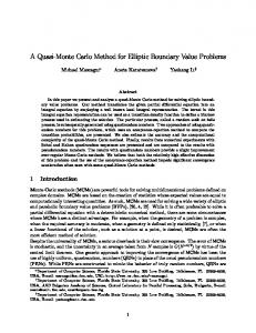
For the first case of interest, as is shown in Fig. 1, at the left end of rods, say s = 0, the position vector RL is given and also the local basis vectors d1L , d2L , d3L . At the right end of rods, say s = L (length of rods), external forces FR and torques MR are exerted. All the given boundary conditions are expressed in the general fixed frame now. However, we still need another fixed reference frame XYZ, the axis of which is related to the direction of the tension of rods and also in which the closed form of the solution of our system is given as seen in Fig. 1. All the given boundary conditions will be represented in this reference frame after it is built. Let us choose the axis Z of the reference frame oriented along the external force exerted at the right end of rods and take the left end of rods as its origin. It is easy to see that the angle between axis Z and the tangent director d3 at the starting point of rods is the initial value of Euler angle β, the cosine of which is equal to z0 . The axis Y will be the cross-product of vector Z and d3L . Then one can easily get the axis X of the reference frame X = Y × Z. Next we can use the local triad given at the left end of rods to determine the initial values of the other two Euler angles, α and γ. To do so we set another local reference frame at the point, say d1L d2L d3L . The axis d3L of the local reference frame coincides with the axis d3L and the axis d2L coincides with the axis Y of the reference frame XYZ. Then we have d1L = d2L × d3L . Accordingly, the three Euler angles of the local reference triad d1 d2 d3 given in the reference frame XYZ areα0 = γ0 = 0, β0 = arccos(z0 ), respectively. One can see that the only difference between the given local frame d1L d2L d3L and local reference frame d1L d2L d3L is a rigid rotation along axis d3L . Thus the initial values of the three Euler angles of the local triad d1L d2L d3L are α0 = 0, β0 = arccos(z0 ), γ0 = γ 0 , respectively, where γ0 is the angle by which the axis d1L is rotated to axis d1L along axis d3L . Now all boundary conditions given at the starting point have been used. And at the other end of rods, the external force condition FR has been used too, because its direction is used for setting the axis Z and its magnitude is equal to one of the four constant system integrals, namely F . In addition at any point of rods, say s, the internal moment Ms can be expressed as Ms = (∆Rs ) × FR + MR

394

L. Shu and A. Weber

Fig. 1. Boundary matching scheme

where ∆Rs = RR − Rs , RR and Rs are the position vector of the right end of rods and the point s, respectively. Projecting both sides of the above equation along axis Z, one can get the constant system integral Mz , Mz = (MR ) · ez However M3 can not be obtained in this way, because ∆Rs can not be determined. Neither the constant system integral H can be determined using the given boundary conditions. But if these two system constants are determined all the descriptive variables of Kirchhoff rods can be determined. Thus we may take them as unknown parameters to be determined. In the following we give a method for finding appropriate values for the two parameters to match the given boundary conditions. So far the only boundary condition that has not been used is the moment exerted at the right end of rods, which can be equivalently written as κ1 (L) − κ1 (L) = 0 κ2 (L) − κ2 (L) = 0 (18) κ3 (L) − κ3 (L) = 0 where κi (L) and κi (L), i=1, 2, 3, represent the curvature along the ith axis at point s = L. The former is determined by using eqn. 2, while the latter is calculated by using the constitutive relationship and the exerted moment there, obtained by the following formulae. κ1 (L) = MR · d1 (L) κ2 (L) = MR · d2 (L) κ3 (L) = MR · d3 (L)/b constructing a function as follows:


395

1 2 2 2 [κ1 (L) − κ1 (L)] + [κ2 (L) − κ2 (L)] + [κ3 (L) − κ3 (L)] 2

(19)

f1 =

One can easily see that it is in fact a function of the constant system integrals M3 and H. In addition—from the definition of the function—one can see that the conditions minimizing the function 19 are necessary and sufficient for eqn. 18 to be fulfilled, and vice versa. Thus the problem of matching the last boundary conditions, eqn. 18, is converted to finding appropriate M3 and H that minimize the function f1 from 19. Because we are going to deal with an unconstraint minimization problem, the two unknown parameters M3 and H could be in the range of the whole real region. However H can not take all real numbers since it can be expressed in term of Euler angles as in [7],

(Mz − M3 z)2 M32 1 2 + (20) + Fz H= (θ ) + 2 b 1 − z2 where θ = dθ . Eqn. 21 indicates that H can only be in some regions of ds the reals. However by observation of eqn. 21, we found that θ can be any real number. Thus we select θ as the other unknown parameter for our minimization scheme in place of H. Since H is a constant system integral which is of course not dependent on arc length, we can extract it at the starting point where the Euler angle β w and P = θ (0) and other necessary parameters are known in this case. Then M3 and P are selected as the unknown parameters for our minimization problem. A global minimization approach can be well chosen to find appropriate values of M3 and P with which the explicit form solution of our system can match the given boundary conditions. We refer to the first example in Sec. 4. 3.2

The Second Case of Boundary Conditions

In this section we use similar technique to deal with another case of boundary conditions. At the left end of rods, say s = 0, the position vector RL is given and also the local triad of the point d1L , d2L , d3L . At the other end of rods only the position vector RR = (xR , yR , zR ) is given, written as, x(L) = x R

y(L) = yR z(L) = zR

(21)

where x(L) y(L) z(L) is the position vector at the right end of rods which is the result of integrating eqn. 3. Similarly we first construct a cost function f2 , 1 2 2 2 (22) [x(L) − xR ] + [y(L) − yR ] + [z(L) − zR ] f2 = 2 According to the definition of the function 22 the conditions that minimize the function 22 are equivalent to the boundary condition in eqn. 21. For this case of boundary conditions we choose Mz , M3 , β0 and P (P = θ (0)) as the unknown parameters to be determined. This case is a little bit more complex than the previous one because all these parameters cannot be determined

396

L. Shu and A. Weber

directly by using the given boundary conditions. The constant system integral F is in this case taken as an external parameter. Then we can examine how the closed form of solution matches the given boundary conditions at different level of tension. When the cost function is evaluated Mz , M3 , β0 and P will be passed to it as input arguments. Similarly we first build a reference frame XYZ. Without loss of generality, we choose the left end of rods as its origin. Then we set the axis Y of the reference frame oriented along the direction that is perpendicular to the tangent director d3L at the left end of rods just like that of Sec. 3.1. The axis Z is set as a vector which will coincide with the tangent director d3L at the left end of rods if it is rotated by angle β0 along axis Y. Then one can easily get X = Y × Z. After the reference frame is obtained, one can similarly determine the other two initial values of Euler angles α0 and γ0 using the local triad given at the left end of rods. Thus the problem of matching the boundary condition, eqn. 21 is converted to solving an unconstrained minimization problem with Mz , M3 , β0 and P as unknown parameters to be determined by minimizing f2 .

4

Example

Our work is motivated by human hair modeling. In the following example we assume that the rods considered will have the physical properties of human hair: the Young’s module of rods is 3.89e10 dyne/cm2 ; the Poisson’s ratio is 0.25; the radius of rods is 0.005 cm [15]. For the example, we consider the first case of boundary conditions in which the left end of a rod is fixed at the origin and the director vectors are also given, d1 = (0.0, 0.0, 1.0), d2 = (1.0, 0.0, 0.0); and at the right end of the rod, external forces and torques are exerted, FR = (0.0, 0.0, -2.0), MR = (0.0, 0.0, 5.0). We will consider several rods with various length in the example, say L= 10cm, 20cm, 30cm, respectively. We use the multidimensional downhill simplex method for our minimization task [16]. Although the algorithm is not a global minimization method, from the definition of our cost function, one can easily know that it is non-negative in the whole real region. It can be inferred that the global minimum of our cost function is zero. Thus we can easily check if the results of the minimization scheme are the desired. In addition, we do not need to evaluate the derivative of the cost function in the minima finder, which can only be calculated numerically in our method. On the other side, we also use a global minimization method for the purpose, called Sigma [17]. However in our experience, it will be very time consuming if we use the global method. The cost function will be evaluated for about several tens of thousands or even hundreds of thousands times. However similar results compared with those of the downhill simplex method were obtained, in which only several hundreds of times of evaluation of the cost function are needed. In Table 1, we give the results of our computations of several rods with different length under the case of boundary conditions. In Fig. 2 (a) to (c), we show the final shape of the rods for three cases.


397

Table 1. Results of our minimization method for the example The CPU times were measured on a Pentium IV 2.2 GHz PC. Length (cm) Values (M3, P) at start Function value Values (M3, P) at end Function value Number of function evaluations Total CPU time (approximate)

10 (-2.0, -2.0)

20 (-0.260, 0.375)

30 (-0.262, 0.375)

5.091

0.03337

0.2223

(-0.2583, -0.3740) 0.0

(-0.26183, 0.37538) 0.0

(-0.2618, 0.3753) 0.0

219

179

220

0.5 sec

0.5 sec

0.5 sec

Fig. 2. The shapes of a rod with a variety of lengths; (a) length: 10 cm; (b) length: 20 cm; (c) length: 30 cm

5

Conclusion

In this paper we presented a symbolic-numeric method for solving various boundary value problems associated with the static Kirchhoff rods. We first expressed the explicit form of solution to the static Kirchhoff rod equations in a form which is easily parameterized by initial values. By combining the parameterized closed form solution with a global minimization scheme we presented a general method in which the problem of solving the boundary value problems associated with static Kirchhoff rods is converted to the problem of solving an unconstrained global minimization problem. Our method can be used to adapt a variety of boundary conditions, as we only need to construct different cost functions for them. An adaptation to other constraints and boundary conditions, e.g. the ones arising from contact between hair fibers, will be a topic of our future research.

398

L. Shu and A. Weber

Acknowledgements. The work was financially supported by Deutsche Forschungsgemeinschaft under grant We 1945/3-1.

References 1. Chin, C.H.K., May, R.L., Connell, H.J.: A numerical model of a towed cable-body system. J. Aust. Math. Soc. 42(B) (2000) 362–384 2. Swigon, D., Coleman, B.D., Tobias, I.: The elastic rod model for DNA and its application to the tertiary structure of DNA minicircles in mononucleosomes. Biop. J. 74 (1998) 2515–2530 3. Colemana, B.D., Olsonb, W.K., Swigonc, D.: Theory of sequence-dependent DNA elasticity. J. Chem. Phys. 118 (2003) 7127–7140 4. Moakher, M., Maddocks, J.H.: A double-strand elastic rod theory. In: Workshop on Atomistic to Continuum Models for Long Molecules and Thin Films. (2001) 5. Coleman, B.D., Swigon, D.: Theory of self-contact in Kirchhoff rods with applications to supercoiling of knotted and unknotted DNA plasmids. Philosophical Transactions: Mathematical, Physical and Engineering Sciences 362 (2004) 1281– 1299 6. Goriely, A., Tabor, M.: Spontaneous helix-hand reversal and tendril perversion in climbing plants. Phys. Rev. Lett. 80 (1998) 1564–1567 7. Nizette, M., Goriely, A.: Towards a classification of Euler-Kirchhoff filaments. Journal of Mathematical Physics 40 (1999) 2830–2866 8. Goriely, A., Nizette, M., Tabor, M.: On the dynamics of elastic strips. Journal of Nonlinear Science 11 (2001) 3–45 9. da Fonseca, A.F., de Aguiar, M.A.M.: Solving the boundary value problem for finite Kirchhoff rods. Physica D 181 (2003) 53–69 10. Thomas, Y.H., Klapper, I., Helen, S.: Romoving the stiffness of curvature in computing 3-d filaments. J. Comp. Phys. 143 (1998) 628–664 11. Rappaport, K.D.: S. Kovalevsky: A mathematical lesson. American Mathematical Monthly 88 (1981) 564–573 12. Goriely, A., Nizettey, M.: Kovalevskaya rods and Kovalevskaya waves. Regu. Chao. Dyna. 5(1) (2000) 95–106 13. Shi, Y., Hearst, J.E.: The Kirchhoff elastic rod, the nonlinear Schroedinger equation and DNA supercoiling. J. Chem. Phys. 101 (1994) 5186–5200 14. Pai, D.K.: STRANDS: Interactive simulation of thin solids using Cosserat models. Computer Graphics Forum 21 (2002) 347–352 EUROGRAPHICS 2002. 15. Robbins, C.R.: Chemical and physical behavior of human hair. Springer (2002) 16. Press, W.H., Teukolsky, S.A., Vetterling, W.T., Flannery, B.P.: Numerical Recipes in C++, Second Edition. Cambridge University Press (2002) 17. Aluffi-Pentini, F., Parisi, V., Zirilli, F.: Sigma — a stochastic-integration global minimization algorithm. ACM Tran. Math. Soft. 14 (1988) 366–380