A Synchrophasor Measurement Algorithm Suitable for Dynamic Applications Jacques Warichet
Tevfik Sezi
Jean-Claude Maun
Universit´e Libre de Bruxelles Brussels, Belgium
[email protected]
Siemens A.G. Nuremberg, Germany
[email protected]
Universit´e Libre de Bruxelles Brussels, Belgium
[email protected]
Abstract - This paper describes a scheme to improve the overall performance of Phasor Measurement Units (PMU), such that the estimated phasors can be used for a wide range of applications in real-time. The main concern is the accuracy and robustness of the phasor estimation outside steadystate, which is strongly influenced by the accuracy of the frequency estimation. The need to complement the phasor data with information about the phasor quality is also emphasized.
Keywords - Phasor measurement, phasor quality assessment, on-line power system stability assessment. 1 Introduction Phasor Measurement Units ability to measure the phase angle of input signals makes them particularly suitable for dynamic events monitoring [1]. However, during serious dynamic events (e.g. losses of synchronism and interarea oscillations), large swings in active power, frequency and other system variables can occur. In that case, the strict definition of a phasor representation is no more valid and measurement accuracy is inevitably lower than in steady-state. 1.1
PMU accuracy specifications
According to the IEEE standard on Synchrophasors [2], the maximum phase-shift accuracy one may need for state estimation, monitoring, control, and relaying of power systems is 0.1◦ . The deviation in amplitude is usually less critical. For that purpose, a Total Vector Error (TVE) has been defined to designate the quality of PMUs: q 2 2 (Xrf − Xr ) + (Xif − Xi ) (1) TVE = Xr2 + Xi2 where Xrf and Xif are the measured values of the phasor real and imaginary parts, as given by the measuring device, and Xr and Xi are the corresponding theoretical values of the input signal at the instant of measurement. The standard requires the TVE to be measured in steadystate and to be lower than 1%. Levels 0 and 1 are then given to the devices depending on the range (in frequency deviations, amplitude and harmonic distortion) where this condition is fullfilled. 1.2
Phasor Measurement and Dynamic Applications
The standard does not include information concerning the accuracy of the estimated phasors in the messages sent to the Phasor Data Concentrator (PDC) and hence to
16th PSCC, Glasgow, Scotland, July 14-18, 2008
the downstreams applications. Furthermore, it suggests that even outside steady-state, the error on the frequency measurement can be neglected and thus an on-line computation of the TVE would prove to be satisfying for all well-designed devices that belong to levels 0 and 1. The authors of this paper do not agree with this statement. Real-time measurement of the frequency may not be free of errors if the frequency varies inside the considered data window, as it is the case for interarea oscillations, where slopes reaching 0.1 to 0.8 Hz/s are possible. Since phasor measurements have a high added value outside steady-state with respect to other measurement techniques, errors in frequency and thus on the phasor must be considered for dynamic applications. Therefore, the authors strongly advise to assess the quality of the computed phasors on-line. Unfortunately, the TVE as defined by equation 1 cannot be computed on the field, since the theoretical phasor is unknown. Another indicator of the phasor quality is thus needed. 1.3 Paper contents The content of this paper is as follows. Section 2 reminds the definition of the phasor and the errors in phasor measurement. Section 3 focuses on frequency measurement, an essential stone in phasor measurement. Section 4 introduces the scheme that aims at improving the PMU accuracy and robustness. Section 5 covers the phasor quality issue and the conclusions come at section 6. 2 Phasor Measurement For a discrete signal x(k), if the DFT (Discrete Fourier Transform) data window contains exactly one cycle of samples, the phasor of fundamental frequency is given by √ N −1 2 X x(k + n − N + 1)e−j2πn/N X(k) = N n=0
(2)
where N is the number of samples and the subscript k represents the last sample index in the data window. The resulting phasor rotates on the complex plane with an angular speed determined by the signal frequency, which can be taken as instantaneous frequency f=
1 arg[X(k + 1)] − arg[X(k)] 2π ∆t
(3)
where arg[X(k)] = tan−1 {Im[X(k)]/Re[X(k)]}. This means that the phasor estimation and frequency estimation are highly correlated to each other. If the design wrongly
Page 1
assumed that sampling rate is an integer multiple of signal frequency, the DFT will produce leakage error on both phasor and frequency measurement. Various solutions exist to match the data window length to the input signal cycle, and thus avoid leakage error. Since this paper supposes that the measuring device has a fixed hardware sampling rate fs , in the order of 10 kHz, software re-sampling will be used so that the data window will always include a fixed amount N of samples for one signal cycle. A feedback loop is used to adjust the re-sampling rate fr by the estimated frequency. 2.1
Error in Phasor Estimation
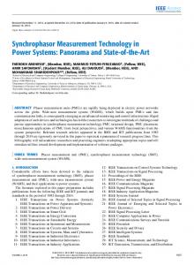
Since phasor measurement is strongly linked to frequency estimation, the phasor measurement accuracy will be strongly influenced by the frequency estimation performance. It has been demonstrated in [3] that the estimation Xf of the actual phasor X is a function of two factors KD and KI , as shown in figure 1. The main component KD rotates slowly at the frequency (f − f0 ), where f is the actual signal frequency and f0 is the estimated frequency used to adapt the re-sampling rate. Its amplitude is close to 1. The second component KI is smaller, equal to 0 if f = f0 , but grows as they differ from each other, and rotates at the frequency (f + f0 ). This unwanted term introduces an incertitude area around the phasor. As a consequence, the estimated phasor of a steady-state signal with f 6= f0 will describe an ellipse on the plane instead of a circle as the actual phasor does. 1
f+f f-f
0
0
KD KI 0.8
0.6
X
KI
KD
0.4
0.2
Xf
2.2 Error in the Measurement Chain Errors in phasor measurement are manifold. They are due to imperfect synchronization, to A/D conversion errors, and to noise and inaccuracies in measurement transformers. While Voltage Transformers errors are lower than 0.5%, Current Transformers have amplitude errors reaching 2%. Calibration techniques are arising to improve this situation. Whereas today’s units internal deviations are neglectable with respect to these values, the synchronization is still a major concern. New technology allows synchronization of the devices with an accuracy higher than 1 µs (0.018 deg at 50 Hz) but the GPS receiver also introduces delays that can lead to a total synchronization error of about 5 µs (0.09 deg). Alltogether, these errors contribute to non-negligeable inaccuracies in the measurement and are as critical as the phasor measurement itself for dynamic applications. 3
Frequency Measurement
Two methods for frequency estimation have been used for this paper. The first method makes use of the relation 3 between frequency and phasor, and operates in closed loop. The second method belongs to the family of signal decomposition methods. Many other methods can be found in the literature. A good summary is given in [5]. The frequency measurement is here based on singlephase signals. Whereas it is more convenient (as explained later) to use the positive sequence component of threephase signals for frequency measurement, it happens that some phases are unusable (single-phase faults and tripping, noise) and that single-phase frequency measurement must be used. 3.1 DFT-based Method (DFTB)
0
−0.2
−0.4 0
25
50
75
100
Frequency (Hz)
Figure 1: Error in phasor computation when the data window length does not fit to the signal cycle: (a) Components KD and KI in the complex plane ; (b) Amplitude of KD (f ) and KI (f ) when f0 = 50 Hz.
The mathematical expression of Xf (k), the estimated phasor at sample k, is given in equation 4. The resampling period Tr is the inverse of the re-sampling rate fr = N f 0 . Xf (k) = KD ·X ·ej2π(f −f0 )kTr +KI ·X ·e−j2π(f +f0 )kTr (4) where KD
=
KI
=
N −1 f −f0 sin(π [f − f0 ] Tr ) · e−jπ N f0 (5) N sin(π [f − f0 ] Tr ) N −1 f +f0 sin(π [f + f0 ] Tr ) · ejπ N f0 (6) N sin(π [f + f0 ] Tr )
The second component KI has an important consequence on the frequency estimation based on the DFT of singlephase signals. The explanation is postponed to the next section.
16th PSCC, Glasgow, Scotland, July 14-18, 2008
Computing the signal instantaneous frequency from relation 3 seems practical because of the simultaneous computation of fundamental phasor and frequency. arg[X]
t
t (ms)
1/2 cycle
Figure 2: Frequency computation using the arguments of the phasors inside a three-cycle data window: (a) One-cycle phasors inside the data window ; (b) Frequency estimation through curve fitting.
However, because of the component KI in relation 4, which is rotating at about twice the signal frequency, an accurate evaluation of the frequency error (f − f0 ) is only possible when the component KI of the used phasors has the same contribution to the deviation. We must then use phasors distant from each other by a multiple of π radians, therefore, about half a cycle. This limits the number of points available to compute the frequency, and imposes the use of data windows of at least one and a half
Page 2
The main advantage of this method is the limited number of operations. Only additional phasors are needed to estimate the frequency. The main drawback is that the computed frequency is a mean value inside the data window and not an instantaneous value. This leads to some delay in the frequency tracking. Another disadvantage is the limited range of the method. If the frequency f is far from f0 in relation 4, the phasor drift will not be close to one turn for every cycle and the KI component will disturb the measure. With the feedback loop, this error will tend to zero but some transition period is needed to settle down to zero error. 3.2
Signal Decomposition Method (SDM)
This method, first presented in [4], uses a group of FIR filters to derive the frequency. After pre-filtering through a band-pass filter with unitary amplitude at the nominal frequency, the input signal is decomposed by an all-pass filter and a low-pass filter. The decomposed signals will then pass through two groups of cascading FIR filters. The frequency is derived from the outputs of the two paths, during which the error brought by filter gains are canceled out. The window length M needed for the pre-filtering is constant and equal to two cycles at nominal frequency.
Figure 3: Block diagram of the signal decomposition method for frequency measurement.
The frequency functions A(Ω) and L(Ω) of the allpass and low-pass filters are: A(Ω)
=
1
L(Ω)
=
1 + cos
µ
¶ M Ω 4
where Ω = 2πf /fs is the normalized frequency, f is the actual frequency and fs is the sampling frequency. As shown in figure 3, the outputs of filters A and L each
16th PSCC, Glasgow, Scotland, July 14-18, 2008
pass through a block C that calculates a value proportional to the square of the signal amplitude, respectively A1 (Ω) and A2 (Ω). Block Q then calculates the quotient A1 (Ω)/A2 (Ω) and block R its square root to provide the ratio of the two calculated amplitudes, XL /XA . This ratio corresponds to the known ratio of the frequencydependent amplification factors of the filters L(Ω) and A(Ω). Hence, µ ¶ XL 4 arccos −1 (8) Ω= M XA 2 Lowpass Allpass
Gain
1.5 1 0.5 0 0
10
20
30
40
50
60
70
80
90
100
10
20
30
40
50
60
70
80
90
100
0 Phase [deg]
cycle. (This is not the case when using the positive sequence component of a three-phase signal, because the KI terms are equal and 120 degrees apart, so they cancel. In this case we could use more points, with more flexible intervals.) With a longer data window, noise rejection will be better but the dynamic response will be slower if the frequency is varying inside the window. For shorter windows, low-pass filtering is needed for satisfactory noise rejection, at the expense of a light delay. For this paper, we choose a two-cycle window. This gives three phasors inside a window and the frequency will be the slope of the fitting curve, similarly to what is shown on figure 2 for a three-cycle data window. The frequency is simply computed by equation 7. µ ¶ 1 dφ − 2πf0 f = f0 + (7) 2π dt
−50 −100 −150 −200 0
Frequency [Hz]
Figure 4: Frequency characteristic of the all-pass and low-pass filters A and L.
The main advantage of this method is that it computes an instantaneous frequency. For phasor measurement, another advantage comes from the separated computations of the phasor and frequency. In the non-causal scheme detailed in the next section, it is possible to use the instantaneous frequency of the signal to re-sample the data and compute the phasor with a high accuracy. This is not possible for the DFT-based method if we do not want to re-sample the same data many times. As drawback, we would mention the group delay of the FIR filters that slows down the dynamic response. More generally, the frequency output is highly sensitive to harmonics and noises so that pre-filter design is critical to the overall performance of this method. (When using three-phase signals, the use of the α component from the Clarke transformation provides some additive smoothing of the noise.) 3.3 Performance Comparison Performance of a frequency measurement method must be evaluated on three criteria: estimation latency, accuracy and robustness. The needed performance indices are thus the following: estimation delay, average error and maximum error [5]. For both methods, a data window of two cycles long has been chosen. In the case of the DFT-based method (called DFTB from now on), it contains three phasors to compute the frequency. On the other hand, two cycles is the needed length for the band-pass filter used by the signal decomposition method (called SDM from now on). Since DFTB calculates the frequency from a linear approximation on three points, we can consider that the computed frequency is closest to the actual frequency at the middle of the window. The delay is then equal to approximately 1 cycle. The noise rejection low-pass filter cares
Page 3
50 49.8 49.6 49.4 49.2 49 48.8 48.6 48.4
SDM DFTB Actual frequency
48.2 48
0
0.2
0.4
0.6
0.8
1
time [s]
Figure 6: Frequency tracking when both amplitude and frequency are time-varying.
4 Scheme for Improving Phasor Measurement Performance
50.5 50.45
(2)
50.4
(1)
50.35 frequency [Hz]
This leads to error decaying as the DC component fades away, with a maximal value of 1.5 mHz for DFTB and 0.5 mHz for SDM.
frequency [Hz]
for a delay which is lower than 1/4 of cycle. In SDM, the delay produced by the FIR filters amounts to 1.5 cycle. The band-pass pre-filter cares for 1 cycle on his own. The filters A and L are 1/2 cycle long and introduce 1/4 of cycle of delay. The compensation block C also adds 1/4 of cycle of delay. For steady-state signals at off-nominal frequency, performance are very close, in the order of 10E-9 mHz for ranges of ±3 Hz around the nominal frequency. For frequency steps, DFTB needs between one and two cycles to eliminate initial errors that are in the order of 5 mHz for a 0.5 Hz step change, whereas SDM needs no additional transition period to settle to the actual frequency. This is illustrated on figure 5. This test is a good indicator of performance but step changes in frequency are not physical because of the mass inertia of the rotating machines of the power system.
50.3
(3)
50.25 50.2 50.15 50.1
SDM DFTB Actual frequency
50.05 50 0
0.02
0.04
0.06
0.08
0.1
time [s]
Figure 5: Performance of the frequency estimation methods during a frequency step of 0.5 Hz: (1) DFTB delay, (2) DFTB settle time, (3) SDM delay.
For signals where both frequency and amplitude are time-varying, like when the system is experiencing oscillations, the frequency estimation is influenced. For example, we consider the following signal, f (t) = A(t) =
49 + cos(2πt) √ 2 (1 + 0.2 sin(3πt))
where the amplitude is modulated by a 1.5 Hz swing and the frequency is modulated by a swing of 1 Hz. The frequency tracking is shown on figure 6. Beyond the delay in frequency dynamics, the amplitude variation does not significantly disturb the measurement except for the first instants where a small discontinuity is observed. The rejection capability against harmonics, noise, DC components and low frequency components, are very similar for both methods. Signals containing odd harmonics, such as that created by power electronics, do not cause any error in frequency estimation. On the other hand, white noise can create substantial errors. A signal with a Signalto-Noise ratio of 40 dB, corresponding to a variance of 1%, gives errors up to 10 mHz for both methods. After system disturbances or switching operations, voltage signals could contain DC components that decay exponentially. Such a signal would be defined, for example, as: √ v(t) = 0.5e−t/0.3 + 2 sin(2πf t + π/6)
16th PSCC, Glasgow, Scotland, July 14-18, 2008
All frequency estimation methods are faced with a trade-off in performances. The accuracy and robustness are linked to the noise rejection capability while the dynamic performances are linked to the estimation latency. Accuracy can be improved by pre-filtering, but then higher delays are introduced and the dynamic performances decrease. Robustness, on the other hand, can be improved through post-processing. To avoid this trade-off and optimize the phasor measurement performances in all circumstances, a flag management scheme is suggested. It allows the signal processing to adapt to the signal characteristics. As a consequence, the robustness and accuracy can be improved without worsening dynamic performance. Before the description of the flag management, let us first have a discussion on the causality of the algorithm, which also influences the PMU performance. 4.1 Algorithm Causality “Causality or causation denotes the relationship between one event (called cause) and another event (called effect) which is the consequence (result) of the first” [6]. For our purpose, the first event is the measurement of the frequency f0 and the effect is te update of the re-sampling rate fr for phasor computation. Because of the inherent latency of all frequency measurement methods, a delay in the adjustment of the resampling rate is unavoidable. However, dynamic performance of phasor measurement can be improved by modifying the causality of the algorithm. Two procedures are possible: Causal algorithm: Priority is set to shorten the delay between sample extraction and phasor computation. The frequency used for re-sampling is the last available estimation of the signal frequency, which corresponds to the actual frequency reigning two to three cycles backward.
Page 4
Various degrees of non-causality can be created, depending on the delay between the data window used for frequency estimation and the data window used for phasor computation. A zero degree means that last sample kf of the data window used for frequency estimation is also the last sample kp of the data window used for phasor computation. A degree one means that there is one cycle at nominal frequency between kf and kp , and so on for higher degrees. Figure 7 illustrates the difference between the causal algorithm and the non-causal algorithm of degree one. For the causal algorithm, there are three cycles between kf and kp . frequency estimation
t
frequency estimation
t
1cycle phasor
1cycle phasor 0
f
fx N
f
fx N
Figure 7: Causality in the update of the re-sampling rate from the frequency of a previous window: (a) Causal algorithm ; (b) Non-causal algorithm of degree 1.
The reader would remark that this delay is a function of the refreshing rate of the estimated frequency. In this paper, this rate has been chosen equal to one cycle at nominal frequency. Another detail can be retained in figure 7. Every onecycle phasor is part of a two-cycle data window. This additional cycle in the window, which is strictly necessary only for the DFT-based method, is needed for the flag management algorithm described next. This has the effect of delaying the frequency update by one more cycle than what seems necessary if we only consider the frequency estimation delay. Figure 8 shows the tracking performance of both the causal algorithm and non-causal algorithms of degree one. This test signal simulates the oscillating behavior of voltage under load/generation imbalance as the consequence of the loss of a major generating unit. The voltage frequency is time-varying and its expression is: £ ¤ f (t) = 47 + 2 1 + 0.4e−t cos(1.5t − 0.1) + 0.2e−7t/10 cos(12t) The choice between causal and non-causal procedures will depend upon the kind of application, privileging either higher accuracy or shorter time-delay. For monitoring purposes, higher delays are not critical. The non-causal algorithm is then preferred because of its higher accuracy. On the other hand, for control and protection applications where time delays must be reduced, the causal algorithm could prove to be the best solution. For Wide Area applications, the delay in PMU data transmission to the PDC
16th PSCC, Glasgow, Scotland, July 14-18, 2008
could be so significant that the non-causal algorithm can be used. 50
Causal update Non causal update Actual frequency
49.8 frequency [Hz]
Non-causal algorithm: In this case, a higher latency is accepted before computing the phasor. With respect to the causal algorithm, later samples are used to compute the window frequency. In that case, the estimated frequency is closer to the actual frequency and the phasor error is reduced.
49.6 49.4 49.2 49 48.8
0
0.5
1
1.5
time [s]
Figure 8: Delay in the update of the sampling rate for phasor computation in the causal and non causal (degree one) algorithms.
4.2 Flag Management (FM) Since PMUs must be able to measure phasors in steady-state as well as during dynamic events and during transient disturbances, it seems natural to adapt the signal processing to the reigning conditions to optimize phasor measurement performances. Therefore, the authors have implemented a flag management algorithm able to assign a tag to each input data window. This tag will then lead to a processing technique best suited to the signal characteristics for frequency and phasor measurement. It is also advised to add this tag to the information accompanying the phasor sent to the applications. Four tags have been defined: Initialization The algorithm has just been switched on, after recovery from the loss of input signal or GPS pulse. Steady-state The input signal is free of distortion (except measurement noise and odd harmonics) and the frequency is stable. Dynamic state The frequency and amplitude of the signal show significant deviations but continuity is preserved, in frequency as well as in phase angle. Fast transient Singular components (jumps, swells, sags), high noise or even harmonics are present. Classification into one of those four tags is done through a complex logic making use of the computation of the one-cycle residue defined by equation 9, N/2
Res1−cycle =
X [x(j) + x(j + N/2)]2 j=1
x(j)2
(9)
where N is the number of samples at frequency fr used for phasor computation. The one-cycle residue compares among them the two halfs of the samples used for phasor computation. If the
Page 5
re-sampling rate fr is exactly equal to N times the signal frequency f , and the signal contains no noise and no even harmonics, then the first half of the samples is the exact opposite of the second half of the samples, and the residue value is equal to zero. Higher values of the residue allow to detect noise (DC component, white noise, even harmonics), frequency variations and singularities. Discrimination between all these effects is made thanks to thresholds for residue values and by inspecting the time evolution of the residues. Residues are also used to switch from threephase to single-phase computation of the signal frequency when there is abnormal noise on one channel. The basic principle is that we can classify the residues associated to steady-sate signals, dynamic signals and transient signals in ascending order. However, some cases are critical and the knowledge of a single residue does not allow to assign the correct tag to the data window. For example, to distinguish a steady-state signal with a high level of noise (SNR below 25 dB) from a signal where the frequency operating point is slowly moving (at a rate lower than 10mHz/s), more robust indicators are needed. This is why we stated at the previous section that the data windows for phasor computation should be two cycles long (at least). We then have three phasors with associated residues, one half cycle apart from each other, and we can use the slope of those three residues and the ratio σ/µ, that is, the variance divided by mean value of the residues, to discriminate between tags in ambiguous cases. An other example of particular importance is the presence of a phase jump due to a disturbance somewhere in the system. The phasor containing the phase jump will be wrong, and so will be the estimated frequency using this data window. It is thus necessary to recognize it. Only the cycle(s) affected by the jump will show a residue far from those of the other cycles. INITIALIZATION
STEADY-STATE
DYNAMIC
Figure 9 shows the four tags given by the flag management algorithm and the possible transitions for adjacent data windows. As specified in table 1, the difference in processing due to the assigned tag occurs during the post-processing of the frequency, before the re-sampling rate is adjusted. For steady-state windows, frequency filtering is done through, first, limiting frequency variations to 5mHz between two consecutive windows, and then by filtering the computed frequency with the last five values. During initialization as well as during dynamic events, the frequency must be followed as closely as possible. On the opposite, for transient events, it is more convenient to block the frequency estimation to avoid large inaccuracies. While for steady-state and dynamic windows the accuracy of the estimated phasors lies inside a limited range, the uncertainty is larger for transient windows. Applications making use of the latter data must take this uncertainty into account to avoid erroneous decisions, especially in the case of on-line applications. Tag
Frequency processing free f filtering free f fixed f
Initialization Steady-state Dynamic Transient
Accuracy uncertainty high low moderate high
Table 1: Processing of the data window according to the tag assigned by the flag management algorithm and uncertainty on the phasor accuracy.
Performance of the flag management (FM) are convincing. Figure 10 shows results obtained with the DFTB method for frequency computation. In steady-state, the noise rejection is radically improved. For a 25dB Signalto-Noise ratio, the error in frequency estimation is reduced from 50 to 2 mHz when using FM. When phase jumps happen, only one phasor is disturbed (high value of the error PME, defined later). The next window already gives an accurate value. This is not the case if FM is not used, because the frequency does not adjust immediately. Unfortunately, no substantial gain in accuracy is obtained during dynamic events (varying frequency), but the transitions are detected and lead to a higher robustness. −3
x 10
50.02 6
TRANSIENT
5 4
50.005 PME
frequency [Hz]
50.01
Figure 9: The four tags given by the flag management and the possible transitions between them.
Without FM With FM
50.015
50
3
49.995 2
The importance of assigning the correct tag to a data window is twofold. Firstly, the processing depends on the tag, as depicted on table 1. Tag changes are limited, that is, some tag transitions between window n and window n + 1 are not allowed. Furthermore, some hysteresis is present to avoid oscillations between tags. Since the processing is different for different tags, it is desirable to have some continuity in the processing method. Secondly, the authors believe that the tag should be included in the message sent to the PDC at the reporting rate. The use of the phasors would then be made in concordance to the expected (if not estimated) accuracy of the phasor.
16th PSCC, Glasgow, Scotland, July 14-18, 2008
49.99 Frequency Estimated without FM Estimated with FM
49.985 49.98 0.2
0.4
0.6
0.8
1 time [s]
1
1.2
1.4
1.6
1.8
1
1.1
1.2
1.3
1.4
1.5
1.6
1.7
1.8
time [s]
Figure 10: Performance of the flag management algorithm: (a) Smoothing of frequency estimation disturbed by noise (SNR of 25dB) during steady-state ; (b) Fast recovering after small discontinuities in the signal.
5 Phasor Quality and Applications The authors believe that the information about phasor quality is essential for the end user. Since phasor accuracy varies strongly depending on the reigning conditions, this quality must be assessed on-line and revealed.
Page 6
5.1 On-Line Assessement of the Phasor Quality Donolo and Centeno [7] have suggested a procedure to compute on-line a Phasor Measurement Error (PME). This method is similar to that used by transient monitors to avoid distance misoperations due to signal distortions. It basically computes the error between the actual samples used for phasor computation with samples reconstructed from the estimated phasor. Let us call s(t) the input signal and g(t, p) the signal reconstructed with the parameters p = [A, f, θ] (the phasor-estimated magnitude, frequency and phase). By weighting the integral of the difference between s and g by the rms value of the input signal, this leads to the expression 10. Z b 1 1 |s(t) − g(t, p)|dt (10) PME = rmsg (b − a) a To reduce the computational burden for on-line computation of the integral, quadrature integration methods are preferred in [7] to methods based on homogeneously distributed samples, like the trapezoidal or the Simpson’s methods. However, the quadrature methods achieve accurate results with about half the computational burden only if a high-speed analog-to-digital converter is available inside the PMU to obtain extra samples that are not homogeneously distributed. Since this converter is not included in all commercially available device, we will apply the trapezoidal method in this paper for the sake of generality. The PME characterizes the phasor accuracy, and is somewhat linked to the tag assigned to the computed phasor. The PME can give wrong values if DC components or harmonics are present at the input. Therefore, filtering of the input signal harmonics is needed to yield a PME that reflects the actual quality of the measured phasors. The reader will note that, whereas the TVE defined by expression 1 measures a total error including synchronizing errors as well as phasor amplitude and angle errors, the PME only includes the phasor errors because the theoretical value of the phasor is not known during field measurements. However, the PME value can be complemented to generate a more realistic estimate of field measurement quality. The synchronization delay of an installed PMU can be evaluated at installation time with high-precision devices. This delay (ranging between 1 and 5 µs) can be included in the phasor quality assessment so that all the errors are considered. Table 2 sets the link between the tag assigned by the FM and the corresponding maximal value of the PME and the TVE (containing only the measurement error). The phasor angle error εdeg is also indicated to provide more insight to the reader. 5.2
Phasor Measurement Applications
The tag given to a phasor, together with the quality indicators such as the PME (or an on-line version of the TVE), allows to restrict the use of phasors of the required accuracy for specific applications. As it was said before, phasors tagged as fast transients have a high uncertainty
16th PSCC, Glasgow, Scotland, July 14-18, 2008
on the accuracy and their use for real-time applications must be the object of care. For example, the use of uncertain data for stability monitoring could deteriorate the confidence of the user (operator) into phasor data. As a consequence, it is preferable not to use these data in certain circumstances. Tag Stead-state Dynamic
Transient
moderate noise (SN R > 25 dB) moderate oscillation (df /dt < 1 Hz/s) strong oscillation (df /dt ∼ = 10 Hz/s) small φ-jump (∆φ < 10◦ ) strong disturbance harmonics, fault
PME 1 E-3
TVE 4 E-3
εdeg 0.02◦
2 E-3
10 E-3
0.05◦
4 E-3
20 E-3
0.3◦
25 E-3
40 E-3
1.5◦
> 0.5
> 0.2
Table 2: Link between the tag assigned by the flag management and the phasor error indicators PME, TVE and angle error.
6 Conclusion This paper emphasizes the need to go one step further than the IEEE standard on Synchrophasors [2]. It suggests that information on the quality of the estimated phasors should be carried together with the phasors so that the downstreams applications are fed with data at the specified accuracy. A flag management algorithm is introduced to tag input data windows as steady-state, dynamic or transient, and adapt the processing to improve phasor estimation accuracy and robustness. References [1] J. Warichet, J.-C. Maun, and T. Sezi, “Real-Time Identification of Interarea Oscillating Modes in Power Systems”, Proc. of the Third Conference on Critical Infrastructures, Alexandria, VA, Sept. 2006. [2] IEEE Standard for Synchrophasors for Power Systems, Mar. 22, 2006. IEEE Std C37.119-2005. [3] M. Koulischer and J.C. Maun, “Considerations about the use of the Discrete Fourier Transform in digital protection relays submitted to large frequency deviations”, Proc. of the International Conference on Power System Protection, pp. 19-42, Singapore, 1989. [4] T. Sezi, “A New Method for Measuring Power System Frequency”, Proc. of the Conference on Transmission and Distribution, New Orleans, 11-16 Apr. 1999. [5] S. Xue, B. Kasztenny, I. Voloh, and D. Oyenuga, “Power System Frequency Measurement for Frequency Relaying”, Proc. of the Western Protective Relay Conference, Spokane, Washington, USA, Oct. 16-18, 2007. [6] M. G. Singh, “Systems & Control Encyclopedia: Theory, Technology, Applications”, Pergamon Press, 1987. [7] M. A. Donolo and V. A. Centeno, “A Fast Quality Assessment Algorithm for Phasor Measurements”, IEEE Trans. Power Delivery, vol. 20, no. 4, pp. 2407-2413, Oct. 2005.
Page 7